Health Insurance Costs¶

In this example, we use a dataset of personal medical costs to create a model to estimate treatment costs.

The columns provided include:

age: age of the primary beneficiary.
sex: insurance contractor’s gender.
bmi: body mass index.
children: number of dependent children covered by health insurance.
smoker: smoker on non-smoker.
region: the beneficiary’s residential area in the US: northeast, southeast, southwest, northwest.
charges: individual medical costs billed by health insurance.

We will follow the data science cycle (Data Exploration - Data Preparation - Data Modeling - Model Evaluation - Model Deployment) to solve this problem.

Initialization¶

This example uses the following version of vastorbit:

import vastorbit as vo

vo.__version__

Connect to VAST. This example uses an existing connection called VASTDSN . For details on how to create a connection, see the Connection tutorial. You can skip the below cell if you already have an established connection.

vo.connect("VASTDSN")

Let’s assign the data to a VastFrame object.

data = vo.read_csv("insurance.csv")

Let’s take a look at the first few entries in the dataset.

data

	123 age Integer 100%	Abc sex Varchar(50) 100%	123 bmi Double 100%	123 children Integer 100%	Abc smoker Varchar(50) 100%	Abc region Varchar(50) 100%	123 charges Double 100%
1	19	female	27.9	0	yes	southwest	16884.924
2	18	male	33.77	1	no	southeast	1725.5523
3	28	male	33.0	3	no	southeast	4449.462
4	33	male	22.705	0	no	northwest	21984.47061
5	32	male	28.88	0	no	northwest	3866.8552
6	31	female	25.74	0	no	southeast	3756.6216
7	46	female	33.44	1	no	southeast	8240.5896
8	37	female	27.74	3	no	northwest	7281.5056
9	37	male	29.83	2	no	northeast	6406.4107
10	60	female	25.84	0	no	northwest	28923.13692
11	25	male	26.22	0	no	northeast	2721.3208
12	62	female	26.29	0	yes	southeast	27808.7251
13	23	male	34.4	0	no	southwest	1826.843
14	56	female	39.82	0	no	southeast	11090.7178
15	27	male	42.13	0	yes	southeast	39611.7577
16	19	male	24.6	1	no	southwest	1837.237
17	52	female	30.78	1	no	northeast	10797.3362
18	23	male	23.845	0	no	northeast	2395.17155
19	56	male	40.3	0	no	southwest	10602.385
20	30	male	35.3	0	yes	southwest	36837.467

Data Exploration¶

Let’s check our dataset for missing values. If we find any, we’ll have to impute them before we create any models.

data.count_percent()

	count	percent
"age"	1338.0	100.0
"sex"	1338.0	100.0
"bmi"	1338.0	100.0
"children"	1338.0	100.0
"smoker"	1338.0	100.0
"region"	1338.0	100.0
"charges"	1338.0	100.0

There aren’t missing any values, so let’s get a summary of the features.

data.describe(method = "all")

	"age"	"bmi"	"children"	"charges"	"sex"	"smoker"	"region"
dtype	integer	double	integer	double	varchar(50)	varchar(50)	varchar(50)
percent	100	100	100	100	100	100	100
count	1338	1338	1338	1338	1338	1338	1338
top	18	32.3	0	1639.5631	male	no	southeast
top_percent	5.157	0.972	42.9	0.149	50.523	79.522	27.205
avg	39.20702541106129	30.66339686098652	1.0949177877429	13270.422265141247	4.989536621823618	2.204783258594918	9.0
stddev	14.04996037921615	6.098186911679015	1.2054927397819142	12110.011236694	1.0003191385687538	0.40369403754561717	0.0
min	18	15.96	0	1121.8739	4	2	9
approx_25%	27	26.465230290032675	0	4686.733574174784	4	2	9
approx_50%	39	30.193182732316227	1	9564.609234800047	5	2	9
approx_75%	51	34.67378366752696	2	16773.739236061592	6	2	9
max	64	53.13	5	63770.42801	6	3	9
range	46	37.17	5	62648.554110000005	2	1	0
empty	[null]	[null]	[null]	[null]	0	0	0

The dataset covers 1338 individuals up to age 64 from four different regions, each with up to six dependent children.

We might find some interesting patterns if we check age distribution, so let’s create a histogram.

data["age"].hist(method = "count", h = 1)

We have a pretty obvious trend here: the 18 and 19 year old age groups are significantly more frequent than any other, older age group. The other ages range from 20 to 30 people.

Before we do anything else, let’s discretize the age column using equal-width binning with a width of 5. Our goal is to see if there are any obvious patterns among the different age groups.

data["age"].discretize(method = "same_width", h = 5)

	Abc age Varchar 100%	Abc sex Varchar(50) 100%	123 bmi Double 100%	123 children Integer 100%	Abc smoker Varchar(50) 100%	Abc region Varchar(50) 100%	123 charges Double 100%
1	[15;19]	female	27.9	0	yes	southwest	16884.924
2	[15;19]	male	33.77	1	no	southeast	1725.5523
3	[25;29]	male	33.0	3	no	southeast	4449.462
4	[30;34]	male	22.705	0	no	northwest	21984.47061
5	[30;34]	male	28.88	0	no	northwest	3866.8552
6	[30;34]	female	25.74	0	no	southeast	3756.6216
7	[45;49]	female	33.44	1	no	southeast	8240.5896
8	[35;39]	female	27.74	3	no	northwest	7281.5056
9	[35;39]	male	29.83	2	no	northeast	6406.4107
10	[60;64]	female	25.84	0	no	northwest	28923.13692
11	[25;29]	male	26.22	0	no	northeast	2721.3208
12	[60;64]	female	26.29	0	yes	southeast	27808.7251
13	[20;24]	male	34.4	0	no	southwest	1826.843
14	[55;59]	female	39.82	0	no	southeast	11090.7178
15	[25;29]	male	42.13	0	yes	southeast	39611.7577
16	[15;19]	male	24.6	1	no	southwest	1837.237
17	[50;54]	female	30.78	1	no	northeast	10797.3362
18	[20;24]	male	23.845	0	no	northeast	2395.17155
19	[55;59]	male	40.3	0	no	southwest	10602.385
20	[30;34]	male	35.3	0	yes	southwest	36837.467

Age probably influences one’s body mass index (BMI), so let’s compare the average of body mass indexes of each age group and look for patterns there. We’ll use a bar graph this time.

data.bar(
    ["age"],
    method = "mean",
    of = "bmi",
)

There’s a pretty clear trend here, and we can say that, in general, older individuals tend to have a greater BMIs.

Let’s check the average number of smokers for each age-group. Before we do, we’ll convert the ‘yes’ and ‘no’ ‘smoker’ values to more convenient boolean values.

import vastorbit.sql.functions as fun

# Applying the decode function
data["smoker_int"] = fun.decode(data["smoker"], "yes", 1, 0)

Now we can plot the average number of smokers for each age group.

data.bar(
    ["age"],
    method = "mean",
    of = "smoker_int",
)

Unfortunately, there’s no obvious relationship between age and smoking habits - none that we can find from this graph, anyway.

Let’s see if we can relate an individual’s smoking habits with their sex.

data.bar(
    ["sex"],
    method = "mean",
    of = "smoker_int",
)

Now we’re getting somewhere! Looks like we have noticeably more male smokers than female ones.

Let’s see how an individual’s BMI relates to their sex.

data.bar(
    ["sex"],
    method = "mean",
    of = "bmi",
)

Males seem to have a slightly higher BMI, but it’d be hard to draw any conclusions from such a small difference.

Going back to our earlier patterns, let’s check the distribution of sexes among age groups and see if the patterns we identified earlier skews toward one of the sexes.

data.pivot_table(["age", "sex"])

It seems that sex is pretty evenly distributed in each age group.

Let’s move onto costs: how much do people tend to spend on medical treatments?

data["charges"].hist(method = "count")

Based on this graph, the majority of insurance holders tend to spend less than 1500 and only a handful of people spend more than 5000.

Encoding¶

Since our features vary in type, let’s start by encoding our categorical features. Remember, we label-encoded smoker from boolean. Let’s label-encode some other features: sex, region, and age groups.

# encoding sex
data["sex"].label_encode()

# encoding region
data["region"].label_encode()

# encoding age (already discretized into a handful of bins above)
data["age"].label_encode()

	123 age Integer 100%	123 sex Integer 100%	123 bmi Double 100%	123 children Integer 100%	Abc smoker Varchar(50) 100%	123 region Integer 100%	123 charges Double 100%	123 smoker_int Integer 100%
1	0	0	27.9	0	yes	3	16884.924	1
2	0	1	33.77	1	no	2	1725.5523	0
3	2	1	33.0	3	no	2	4449.462	0
4	3	1	22.705	0	no	1	21984.47061	0
5	3	1	28.88	0	no	1	3866.8552	0
6	3	0	25.74	0	no	2	3756.6216	0
7	6	0	33.44	1	no	2	8240.5896	0
8	4	0	27.74	3	no	1	7281.5056	0
9	4	1	29.83	2	no	0	6406.4107	0
10	9	0	25.84	0	no	1	28923.13692	0
11	2	1	26.22	0	no	0	2721.3208	0
12	9	0	26.29	0	yes	2	27808.7251	1
13	1	1	34.4	0	no	3	1826.843	0
14	8	0	39.82	0	no	2	11090.7178	0
15	2	1	42.13	0	yes	2	39611.7577	1
16	0	1	24.6	1	no	3	1837.237	0
17	7	0	30.78	1	no	0	10797.3362	0
18	1	1	23.845	0	no	0	2395.17155	0
19	8	1	40.3	0	no	3	10602.385	0
20	3	1	35.3	0	yes	3	36837.467	1

Before going further, let’s check the correlation of the variables with the predictor charges.

data.corr(focus = "charges")

data.to_db("insurance.final_ins_data", relation_type = "table")

Predicting insurance charges¶

Since our response variable is continuous, we can use regression to predict it. For this example, let’s use a Random Forest model.

from vastorbit.machine_learning.vast.ensemble import RandomForestRegressor

# define the random forest model
rf_model = RandomForestRegressor(
    n_estimators = 5,
    max_depth = 3,
)

# train the model
rf_model.fit(
    data,
    X = ["age", "sex", "bmi", "children", "smoker_int", "region"],
    y = "charges",
)

We can create a regression report to check our model’s performance.

rf_model.report()

	value
explained_variance	0.8585266043359364
max_error	24659.68335406437
median_absolute_error	1647.8091462821956
mean_absolute_error	2652.973237504626
mean_squared_error	20733456.258315813
root_mean_squared_error	4553.400515912892
r2	0.8585160035229124
r2_adj	0.8578782093990487
aic	22555.790701502156
bic	22592.02532545013

The results seem to be quite good! We have an explained variance around 0.8. Let’s plot the predicted values and compare them to the real ones.

# plot the predicted values and real ones
result = rf_model.predict(
    data,
    name = "pred_charges",
)

# add an index
result["id"] = "ROW_NUMBER() OVER()"

# plot them along the id
result.plot(
    ts = "id",
    columns = ['charges', 'pred_charges'],
)

data.to_db("insurance.final_ins_data", relation_type = "table")

Now, let’s examine the importance of each feature for this model. Ours is a random forest model, so we can use the built-in VAST function to calculate the importance of each predictor with Mean Decrease in Impurity (MDI).

# feature importance for our random forest model
rf_model.features_importance()

data.to_db("final_ins_data", relation_type = "table")

rf_model.features_importance(show = False)

	importance	sign
smoker_int	0.7112212269065885	1.0
bmi	0.17673800620302976	1.0
age	0.10824468672692625	1.0
children	0.003796080163455459	1.0
sex	0.0	0.0
region	0.0	0.0

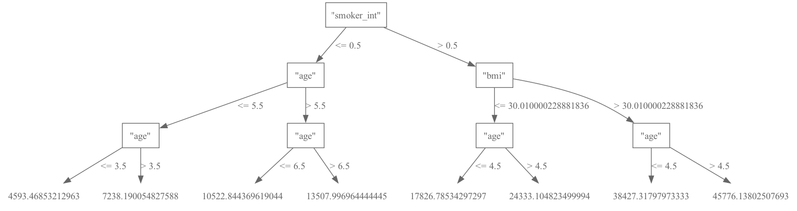
We can examine how our model works by visualizing one of the trees in our Random Forest.

# plot one of the trees comprising the forest
rf_model.plot_tree(tree_id = 3)

_images/examples_insurance_table_rf_tree.png

What affects medical costs?¶

We have a couple ways to approach this question. First, let’s see what features are linearly correlated with the cost.

It seems that smoking habits have a significant effect on medical costs. Next in line comes BMI, the number of dependents, and sex.

As one might expect, the correlation between charges and region is almost 0.

Now, let’s see what we can learn from a stepwise model with backward elimination using Bayesian information criterion (BIC) as a selection criteria.

from vastorbit.machine_learning.vast.linear_model import LinearRegression

model = LinearRegression()

# backward
from vastorbit.machine_learning.model_selection import stepwise

stepwise(
    model,
    input_relation = data,
    direction = "backward",
    X = ["age","sex", "bmi", "children", "smoker_int", "region"],
    y = "charges",
)

	features	bic	change	variable	importance
0	['region', 'sex', 'children', 'bmi', 'age', 'smoker_int']	28811.737130133086	[null]	[null]	0.0
1	['sex', 'children', 'bmi', 'age', 'smoker_int']	28827.22335983746	+	"region"	100.0
2	['region', 'children', 'bmi', 'age', 'smoker_int']	28810.06683163958	-	"sex"	0.0
3	['region', 'bmi', 'age', 'smoker_int']	28757.562416450593	-	"children"	0.0
4	['region', 'age', 'smoker_int']	27654.092097818455	-	"bmi"	0.0
5	['region', 'smoker_int']	26847.61591803939	-	"age"	0.0
6	['region']	25173.12462253033	-	"smoker_int"	0.0

From here we see that, again, the same features have similarly significant effects on medical costs.

Conclusion¶

In this example, we used several methods to identify the primary factors that affect one’s insurance costs.