vastorbit.machine_learning.vast.ensemble.GradientBoostingClassifier¶

class vastorbit.machine_learning.vast.ensemble.GradientBoostingClassifier(name: str = None, overwrite_model: bool = False, **kwargs)¶

Creates an GradientBoostingClassifier object using scikit-learn for training and the scalability of VAST DataBase for the inferences.

Parameters:

name (str, optional) – Name of the model. The model is stored in the database.
overwrite_model (bool, optional) – If set to True, training a model with the same name as an existing model overwrites the existing model.
**kwargs (scikit-learn model parameters.)

Variables:

created (Many attributes are)
phase. (during the fitting)
trees_ (list of BinaryTreeClassifier) – Tree models are instances of ` BinaryTreeClassifier, each possessing various attributes. For more detailed information, refer to the documentation for BinaryTreeClassifier.
feature_importances_ (numpy.array) – The importance of features. It is calculated using the average gain of each tree. To determine the final score, vastorbit sums the scores of each tree, normalizes them and applies an activation function to scale them. It is necessary to use the features_importance() method to compute it initially, and the computed values will be subsequently utilized for subsequent calls.
feature_importances_trees_ (dict of numpy.array) – Each element of the array represents the feature importance of tree i. The importance of features is calculated using the average gain of each tree. It is necessary to use the features_importance() method to compute it initially, and the computed values will be subsequently utilized for subsequent calls.
logodds_ (numpy.array) – The log-odds. It quantifies the logarithm of the odds ratio, providing a measure of the likelihood of an event occurring.
eta_ (float) – The learning rate, is a crucial hyperparameter in machine learning algorithms. It determines the step size at each iteration during the model training process. A well-chosen learning rate is essential for achieving optimal convergence and preventing overshooting or slow convergence in the training phase. Adjusting the learning rate is often necessary to strike a balance between model accuracy and computational efficiency.
n_estimators_ (int) – The number of model estimators.
classes_ (numpy.array) – The classes labels.
note:: (..) – All attributes can be accessed using the get_attributes() method.

Examples

The following examples provide a basic understanding of usage. For more detailed examples, please refer to the Machine Learning or the Examples section on the website.

Important

Many tree-based models inherit from the GradientBoosting base class, and it’s recommended to use it directly for access to a wider range of options.

Load data for machine learning¶

We import vastorbit:

import vastorbit as vo

Hint

By assigning an alias to vastorbit, we mitigate the risk of code collisions with other libraries. This precaution is necessary because vastorbit uses commonly known function names like “average” and “median”, which can potentially lead to naming conflicts. The use of an alias ensures that the functions from vastorbit are used as intended without interfering with functions from other libraries.

For this example, we will use the winequality dataset.

import vastorbit.datasets as vod

data = vod.load_winequality()

	123 fixed_acidity Decimal(6, 3)	123 volatile_acidity Decimal(7, 4)	123 citric_acid Decimal(6, 3)	123 residual_sugar Decimal(7, 3)	123 chlorides Double	123 free_sulfur_dioxide Decimal(7, 2)	123 total_sulfur_dioxide Decimal(7, 2)	123 density Double	123 ph Decimal(6, 3)	123 sulphates Decimal(6, 3)	123 alcohol Double	123 quality Integer	123 good Integer	Abc color Varchar(20)
1	6.3	0.67	0.48	12.6	0.052	57.0	222.0	0.9979	3.17	0.52	9.3	6	0	white
2	7.4	0.4	0.29	5.4	0.044	31.0	122.0	0.994	3.3	0.5	11.1	8	1	white
3	7.1	0.26	0.31	2.2	0.044	29.0	128.0	0.9937	3.34	0.64	10.9	8	1	white
4	9.0	0.31	0.48	6.6	0.043	11.0	73.0	0.9938	2.9	0.38	11.6	5	0	white
5	6.3	0.39	0.24	6.9	0.069	9.0	117.0	0.9942	3.15	0.35	10.2	4	0	white
6	8.2	0.22	0.36	6.8	0.034	12.0	90.0	0.9944	3.01	0.38	10.5	8	1	white
7	7.1	0.19	0.28	3.6	0.033	16.0	78.0	0.993	2.91	0.78	11.4	6	0	white
8	7.3	0.25	0.36	13.1	0.05	35.0	200.0	0.9986	3.04	0.46	8.9	7	1	white
9	7.9	0.2	0.34	1.2	0.04	29.0	118.0	0.9932	3.14	0.41	10.6	6	0	white
10	7.1	0.26	0.32	5.9	0.037	39.0	97.0	0.9934	3.31	0.4	11.6	6	0	white
11	7.0	0.2	0.34	5.7	0.035	32.0	83.0	0.9928	3.19	0.46	11.5	6	0	white
12	6.9	0.3	0.33	4.1	0.035	26.0	155.0	0.9925	3.25	0.79	12.3	8	1	white
13	8.1	0.29	0.49	7.1	0.042	22.0	124.0	0.9944	3.14	0.41	10.8	6	0	white
14	5.8	0.17	0.3	1.4	0.037	55.0	130.0	0.9909	3.29	0.38	11.3	6	0	white
15	5.9	0.415	0.02	0.8	0.038	22.0	63.0	0.9932	3.36	0.36	9.3	5	0	white
16	6.6	0.23	0.26	1.3	0.045	16.0	128.0	0.9934	3.36	0.6	10.0	6	0	white
17	8.6	0.55	0.35	15.55	0.057	35.5	366.5	1.0001	3.04	0.63	11.0	3	0	white
18	6.9	0.35	0.74	1.0	0.044	18.0	132.0	0.992	3.13	0.55	10.2	5	0	white
19	7.6	0.14	0.74	1.6	0.04	27.0	103.0	0.9916	3.07	0.4	10.8	7	1	white
20	9.2	0.28	0.49	11.8	0.042	29.0	137.0	0.998	3.1	0.34	10.1	4	0	white
21	6.2	0.18	0.49	4.5	0.047	17.0	90.0	0.9919	3.27	0.37	11.6	6	0	white
22	5.3	0.165	0.24	1.1	0.051	25.0	105.0	0.9925	3.32	0.47	9.1	5	0	white
23	9.8	0.25	0.74	10.0	0.056	36.0	225.0	0.9977	3.06	0.43	10.0	4	0	white
24	8.1	0.29	0.49	7.1	0.042	22.0	124.0	0.9944	3.14	0.41	10.8	6	0	white
25	6.8	0.22	0.49	0.9	0.052	26.0	128.0	0.991	3.25	0.35	11.4	6	0	white
26	7.2	0.22	0.49	1.0	0.045	34.0	140.0	0.99	3.05	0.34	12.7	6	0	white
27	7.4	0.25	0.49	1.1	0.042	35.0	156.0	0.9917	3.13	0.55	11.3	5	0	white
28	8.2	0.18	0.49	1.1	0.033	28.0	81.0	0.9923	3.0	0.68	10.4	7	1	white
29	6.1	0.22	0.49	1.5	0.051	18.0	87.0	0.9928	3.3	0.46	9.6	5	0	white
30	7.0	0.39	0.24	1.0	0.048	8.0	119.0	0.9923	3.0	0.31	10.1	4	0	white
31	6.1	0.22	0.49	1.5	0.051	18.0	87.0	0.9928	3.3	0.46	9.6	5	0	white
32	6.5	0.36	0.49	2.9	0.03	16.0	94.0	0.9902	3.1	0.49	12.1	7	1	white
33	7.1	0.29	0.49	1.2	0.031	32.0	99.0	0.9893	3.07	0.33	12.2	6	0	white
34	7.4	0.25	0.49	1.1	0.042	35.0	156.0	0.9917	3.13	0.55	11.3	5	0	white
35	6.9	0.23	0.24	14.2	0.053	19.0	94.0	0.9982	3.17	0.5	9.6	5	0	white
36	8.5	0.56	0.74	17.85	0.051	51.0	243.0	1.0005	2.99	0.7	9.2	5	0	white
37	8.2	0.18	0.49	1.1	0.033	28.0	81.0	0.9923	3.0	0.68	10.4	7	1	white
38	6.3	0.23	0.49	7.1	0.05	67.0	210.0	0.9951	3.23	0.34	9.5	5	0	white
39	6.1	0.25	0.49	7.6	0.052	67.0	226.0	0.9956	3.16	0.47	8.9	5	0	white
40	7.2	0.26	0.74	13.6	0.05	56.0	162.0	0.998	3.03	0.44	8.8	5	0	white
41	7.2	0.31	0.24	1.4	0.057	17.0	117.0	0.9928	3.16	0.35	10.5	5	0	white
42	8.0	0.25	0.49	1.2	0.061	27.0	117.0	0.9938	3.08	0.34	9.4	5	0	white
43	7.0	0.18	0.49	5.3	0.04	34.0	125.0	0.9914	3.24	0.4	12.2	6	0	white
44	7.8	0.43	0.49	13.0	0.033	37.0	158.0	0.9955	3.14	0.35	11.3	6	0	white
45	8.3	0.2	0.74	4.45	0.044	33.0	130.0	0.9924	3.25	0.42	12.2	6	0	white
46	6.3	0.27	0.49	1.2	0.063	35.0	92.0	0.9911	3.38	0.42	12.2	6	0	white
47	7.4	0.16	0.49	1.2	0.055	18.0	150.0	0.9917	3.23	0.47	11.2	6	0	white
48	7.4	0.16	0.49	1.2	0.055	18.0	150.0	0.9917	3.23	0.47	11.2	6	0	white
49	6.9	0.19	0.49	6.6	0.036	49.0	172.0	0.9932	3.2	0.27	11.5	6	0	white
50	7.8	0.43	0.49	13.0	0.033	37.0	158.0	0.9955	3.14	0.35	11.3	6	0	white
51	7.2	0.4	0.49	1.1	0.048	11.0	138.0	0.9929	3.01	0.42	9.3	5	0	white
52	7.8	0.43	0.49	13.0	0.033	37.0	158.0	0.9955	3.14	0.35	11.3	6	0	white
53	7.6	0.52	0.49	14.0	0.034	37.0	156.0	0.9958	3.14	0.38	11.8	7	1	white
54	8.3	0.21	0.49	19.8	0.054	50.0	231.0	1.0012	2.99	0.54	9.2	5	0	white
55	6.9	0.34	0.74	11.2	0.069	44.0	150.0	0.9968	3.0	0.81	9.2	5	0	white
56	6.3	0.27	0.49	1.2	0.063	35.0	92.0	0.9911	3.38	0.42	12.2	6	0	white
57	8.3	0.2	0.74	4.45	0.044	33.0	130.0	0.9924	3.25	0.42	12.2	6	0	white
58	7.1	0.22	0.74	2.7	0.044	42.0	144.0	0.991	3.31	0.41	12.2	6	0	white
59	7.9	0.11	0.49	4.5	0.048	27.0	133.0	0.9946	3.24	0.42	10.6	6	0	white
60	8.5	0.17	0.74	3.6	0.05	29.0	128.0	0.9928	3.28	0.4	12.4	6	0	white
61	6.4	0.145	0.49	5.4	0.048	54.0	164.0	0.9946	3.56	0.44	10.8	6	0	white
62	7.4	0.16	0.49	1.2	0.055	18.0	150.0	0.9917	3.23	0.47	11.2	6	0	white
63	8.3	0.19	0.49	1.2	0.051	11.0	137.0	0.9918	3.06	0.46	11.0	6	0	white
64	8.0	0.44	0.49	9.1	0.031	46.0	151.0	0.9926	3.16	0.27	12.7	8	1	white
65	7.0	0.2	0.74	0.8	0.044	19.0	163.0	0.9931	3.46	0.53	10.2	5	0	white
66	6.9	0.19	0.49	6.6	0.036	49.0	172.0	0.9932	3.2	0.27	11.5	6	0	white
67	7.1	0.25	0.49	3.0	0.03	30.0	96.0	0.9903	3.13	0.39	12.3	7	1	white
68	6.5	0.24	0.24	1.6	0.046	15.0	60.0	0.9928	3.19	0.39	9.8	5	0	white
69	7.2	0.4	0.49	1.1	0.048	11.0	138.0	0.9929	3.01	0.42	9.3	5	0	white
70	7.6	0.52	0.49	14.0	0.034	37.0	156.0	0.9958	3.14	0.38	11.8	7	1	white
71	7.8	0.43	0.49	13.0	0.033	37.0	158.0	0.9955	3.14	0.35	11.3	6	0	white
72	7.8	0.21	0.49	1.35	0.052	6.0	48.0	0.9911	3.15	0.28	11.4	5	0	white
73	7.0	0.2	0.49	5.9	0.038	39.0	128.0	0.9938	3.21	0.48	10.8	6	0	white
74	6.9	0.25	0.24	3.6	0.057	13.0	85.0	0.9942	2.99	0.48	9.5	4	0	white
75	7.2	0.08	0.49	1.3	0.05	18.0	148.0	0.9945	3.46	0.44	10.2	6	0	white
76	7.1	0.85	0.49	8.7	0.028	40.0	184.0	0.9962	3.22	0.36	10.7	5	0	white
77	7.6	0.51	0.24	1.2	0.04	10.0	104.0	0.992	3.05	0.29	10.8	6	0	white
78	7.9	0.22	0.24	4.6	0.044	39.0	159.0	0.9927	2.99	0.28	11.5	6	0	white
79	7.7	0.16	0.49	2.0	0.056	20.0	124.0	0.9948	3.32	0.49	10.7	6	0	white
80	7.2	0.08	0.49	1.3	0.05	18.0	148.0	0.9945	3.46	0.44	10.2	6	0	white
81	6.6	0.25	0.24	1.7	0.048	26.0	124.0	0.9942	3.37	0.6	10.1	6	0	white
82	6.7	0.16	0.49	2.4	0.046	57.0	187.0	0.9952	3.62	0.81	10.4	6	0	white
83	6.9	0.25	0.24	3.6	0.057	13.0	85.0	0.9942	2.99	0.48	9.5	4	0	white
84	7.5	0.32	0.24	4.6	0.053	8.0	134.0	0.9958	3.14	0.5	9.1	3	0	white
85	7.4	0.28	0.49	1.5	0.034	20.0	126.0	0.9918	2.98	0.39	10.6	6	0	white
86	6.2	0.15	0.49	0.9	0.033	17.0	51.0	0.9932	3.3	0.7	9.4	6	0	white
87	6.7	0.25	0.74	19.4	0.054	44.0	169.0	1.0004	3.51	0.45	9.8	6	0	white
88	6.5	0.26	0.74	13.3	0.044	68.0	224.0	0.9972	3.18	0.54	9.5	6	0	white
89	7.9	0.16	0.74	17.85	0.037	52.0	187.0	0.9998	2.99	0.41	9.3	5	0	white
90	5.6	0.185	0.49	1.1	0.03	28.0	117.0	0.9918	3.55	0.45	10.3	6	0	white
91	7.5	0.2	0.49	1.3	0.031	8.0	97.0	0.9918	3.06	0.62	11.1	5	0	white
92	8.0	0.3	0.49	9.4	0.046	47.0	188.0	0.9964	3.14	0.48	10.0	5	0	white
93	8.0	0.34	0.49	9.0	0.033	39.0	180.0	0.9936	3.13	0.38	12.3	8	1	white
94	7.7	0.35	0.49	8.65	0.033	42.0	186.0	0.9931	3.14	0.38	12.4	8	1	white
95	7.6	0.29	0.49	9.6	0.03	45.0	197.0	0.9938	3.13	0.38	12.3	7	1	white
96	6.7	0.62	0.24	1.1	0.039	6.0	62.0	0.9934	3.41	0.32	10.4	5	0	white
97	6.8	0.27	0.49	1.2	0.044	35.0	126.0	0.99	3.13	0.48	12.1	7	1	white
98	7.7	0.27	0.49	1.8	0.041	23.0	86.0	0.9914	3.16	0.42	12.5	6	0	white
99	6.7	0.51	0.24	2.1	0.043	14.0	155.0	0.9904	3.22	0.6	13.0	6	0	white
100	7.4	0.19	0.49	9.3	0.03	26.0	132.0	0.994	2.99	0.32	11.0	7	1	white

Rows: 1-100 | Columns: 14

Note

vastorbit offers a wide range of sample datasets that are ideal for training and testing purposes. You can explore the full list of available datasets in the Datasets, which provides detailed information on each dataset and how to use them effectively. These datasets are invaluable resources for honing your data analysis and machine learning skills within the vastorbit environment.

You can easily divide your dataset into training and testing subsets using the VastFrame.train_test_split() method. This is a crucial step when preparing your data for machine learning, as it allows you to evaluate the performance of your models accurately.

data = vod.load_winequality()
train, test = data.train_test_split(test_size = 0.2)

Warning

In this case, vastorbit utilizes seeded randomization to guarantee the reproducibility of your data split. However, please be aware that this approach may lead to reduced performance. For a more efficient data split, you can use the VastFrame.to_db() method to save your results into tables or temporary tables. This will help enhance the overall performance of the process.

Balancing the Dataset¶

In vastorbit, balancing a dataset to address class imbalances is made straightforward through the balance() function within the preprocessing module. This function enables users to rectify skewed class distributions efficiently. By specifying the target variable and setting parameters like the method for balancing, users can effortlessly achieve a more equitable representation of classes in their dataset. Whether opting for over-sampling, under-sampling, or a combination of both, vastorbit’s balance() function streamlines the process, empowering users to enhance the performance and fairness of their machine learning models trained on imbalanced data.

To balance the dataset, use the following syntax.

from vastorbit.machine_learning.vast.preprocessing import balance

balanced_train = balance(
    name = "my_schema.train_balanced",
    input_relation = train,
    y = "good",
    method = "hybrid",
)

Note

With this code, a table named train_balanced is created in the my_schema schema. It can then be used to train the model. In the rest of the example, we will work with the full dataset.

Hint

Balancing the dataset is a crucial step in improving the accuracy of machine learning models, particularly when faced with imbalanced class distributions. By addressing disparities in the number of instances across different classes, the model becomes more adept at learning patterns from all classes rather than being biased towards the majority class. This, in turn, enhances the model’s ability to make accurate predictions for under-represented classes. The balanced dataset ensures that the model is not dominated by the majority class and, as a result, leads to more robust and unbiased model performance. Therefore, by employing techniques such as over-sampling, under-sampling, or a combination of both during dataset preparation, practitioners can significantly contribute to achieving higher accuracy and better generalization of their machine learning models.

Model Initialization¶

First we import the GradientBoostingClassifier model:

from vastorbit.machine_learning.vast import GradientBoostingClassifier

Then we can create the model:

model = GradientBoostingClassifier(
    n_estimators = 3,
    max_depth = 3,
    nbins = 6,
    split_proposal_method = 'global',
    tol = 0.001,
    learning_rate = 0.1,
    min_split_loss = 0,
    weight_reg = 0,
    sample = 0.7,
    col_sample_by_tree = 1,
    col_sample_by_node = 1,
)

Important

The model name is crucial for the model management system and versioning. It’s highly recommended to provide a name if you plan to reuse the model later.

Model Training¶

We can now fit the model:

model.fit(
    train,
    [
        "fixed_acidity",
        "volatile_acidity",
        "citric_acid",
        "residual_sugar",
        "chlorides",
        "density",
    ],
    "good",
    test,
)

Important

To train a model, you can directly use the VastFrame or the name of the relation stored in the database. The test set is optional and is only used to compute the test metrics. In vastorbit, we don’t work using X matrices and y vectors. Instead, we work directly with lists of predictors and the response name.

Features Importance¶

We can conveniently get the features importance:

result = model.features_importance()

Note

In models such as GradientBoosting, feature importance is calculated using the average gain of each tree. To determine the final score, vastorbit sums the scores of each tree, normalizes them and applies an activation function to scale them.

Metrics¶

We can get the entire report using:

model.report()

	value
auc	0.0
prc_auc	0.0
accuracy	0.0
log_loss	0.21525744989987353
precision	0.0
recall	0.0
f1_score	0.0
mcc	0.0
informedness	-1.0
markedness	-1.0
csi	0.0

Rows: 1-11 | Columns: 2

Important

Most metrics are computed using a single SQL query, but some of them might require multiple SQL queries. Selecting only the necessary metrics in the report can help optimize performance. E.g. model.report(metrics = ["auc", "accuracy"]).

For classification models, we can easily modify the cutoff to observe the effect on different metrics:

model.report(cutoff = 0.2)

	value
auc	0.0
prc_auc	0.0
accuracy	0.0
log_loss	0.21568009462021687
precision	0.0
recall	0.0
f1_score	0.0
mcc	0.0
informedness	-1.0
markedness	-1.0
csi	0.0

Rows: 1-11 | Columns: 2

You can also use the score() function to compute any classification metric. The default metric is the accuracy:

model.score()

Prediction¶

Prediction is straight-forward:

model.predict(
    test,
    [
        "fixed_acidity",
        "volatile_acidity",
        "citric_acid",
        "residual_sugar",
        "chlorides",
        "density",
    ],
    "prediction",
)

	123 fixed_acidity Decimal(6, 3)	123 volatile_acidity Decimal(7, 4)	123 citric_acid Decimal(6, 3)	123 residual_sugar Decimal(7, 3)	123 chlorides Double	123 free_sulfur_dioxide Decimal(7, 2)	123 total_sulfur_dioxide Decimal(7, 2)	123 density Double	123 ph Decimal(6, 3)	123 sulphates Decimal(6, 3)	123 alcohol Double	123 quality Integer	123 good Integer	Abc color Varchar(20)	123 seedrand Decimal(26, 6)	123 prediction Decimal(11, 1)
1	6.8	0.37	0.51	11.8	0.044	62.0	163.0	0.9976	3.19	0.44	8.8	5	0	white	0.12	1.0
2	7.2	0.25	0.39	18.95	0.038	42.0	155.0	0.9999	2.97	0.47	9.0	6	0	white	0.1	1.0
3	7.3	0.28	0.36	12.7	0.04	38.0	140.0	0.998	3.3	0.79	9.6	6	0	white	0.07	1.0
4	7.0	0.22	0.31	2.7	0.03	41.0	136.0	0.9898	3.16	0.37	12.7	7	1	white	0.04	1.0
5	7.0	0.21	0.28	8.6	0.045	37.0	221.0	0.9954	3.25	0.54	10.4	6	0	white	0.13	1.0
6	6.9	0.2	0.37	6.2	0.027	24.0	97.0	0.992	3.38	0.49	12.2	7	1	white	0.13	1.0
7	6.6	0.16	0.32	1.4	0.035	49.0	186.0	0.9906	3.35	0.64	12.4	8	1	white	0.1	1.0
8	6.5	0.41	0.24	14.0	0.048	24.0	113.0	0.9982	3.44	0.53	9.8	6	0	white	0.02	1.0
9	6.0	0.37	0.32	1.0	0.053	31.0	218.5	0.9924	3.29	0.72	9.8	6	0	white	0.02	1.0
10	7.1	0.21	0.27	8.6	0.056	26.0	111.0	0.9956	2.95	0.52	9.5	5	0	white	0.06	1.0
11	7.0	0.14	0.32	9.0	0.039	54.0	141.0	0.9956	3.22	0.43	9.4	6	0	white	0.12	1.0
12	7.0	0.22	0.28	1.5	0.037	29.0	115.0	0.9927	3.11	0.55	10.5	6	0	white	0.16	1.0
13	7.1	0.55	0.13	1.7	0.073	21.0	165.0	0.994	2.97	0.58	9.2	6	0	white	0.16	1.0
14	6.7	0.47	0.34	8.9	0.043	31.0	172.0	0.9964	3.22	0.6	9.2	5	0	white	0.07	1.0
15	6.2	0.37	0.3	6.6	0.346	79.0	200.0	0.9954	3.29	0.58	9.6	5	0	white	0.08	1.0
16	6.0	0.16	0.37	1.5	0.025	43.0	117.0	0.9928	3.46	0.51	9.7	6	0	white	0.07	1.0
17	7.0	0.28	0.36	1.0	0.035	8.0	70.0	0.9899	3.09	0.46	12.1	6	0	white	0.14	1.0
18	7.1	0.23	0.39	1.6	0.032	12.0	65.0	0.9898	3.25	0.4	12.7	7	1	white	0.1	1.0
19	5.7	0.44	0.13	7.0	0.025	28.0	173.0	0.9913	3.33	0.48	12.5	6	0	white	0.06	1.0
20	7.2	0.4	0.62	10.8	0.041	70.0	189.0	0.9976	3.08	0.49	8.6	4	0	white	0.15	1.0
21	7.2	0.28	0.54	16.7	0.045	54.0	200.0	0.999	3.08	0.49	9.5	6	0	white	0.02	1.0
22	6.8	0.19	0.58	14.2	0.038	51.0	164.0	0.9975	3.12	0.48	9.6	6	0	white	0.0	1.0
23	7.3	0.26	0.36	5.2	0.04	31.0	141.0	0.9931	3.16	0.59	11.0	6	0	white	0.06	1.0
24	7.8	0.28	0.32	9.0	0.036	34.0	115.0	0.9952	3.17	0.39	10.3	7	1	white	0.01	1.0
25	6.8	0.18	0.37	1.6	0.055	47.0	154.0	0.9934	3.08	0.45	9.1	5	0	white	0.12	1.0
26	7.4	0.15	0.42	1.7	0.045	49.0	154.0	0.992	3.0	0.6	10.4	6	0	white	0.03	1.0
27	5.2	0.36	0.02	1.6	0.031	24.0	104.0	0.9896	3.44	0.35	12.2	6	0	white	0.06	1.0
28	6.1	0.24	0.3	1.5	0.045	22.0	61.0	0.992	3.31	0.54	10.4	5	0	white	0.17	1.0
29	6.8	0.25	0.24	4.55	0.053	41.0	211.0	0.9955	3.37	0.67	9.5	6	0	white	0.09	1.0
30	6.8	0.28	0.17	13.9	0.047	49.0	162.0	0.9983	3.21	0.51	9.0	6	0	white	0.19	1.0
31	7.0	0.3	0.51	13.6	0.05	40.0	168.0	0.9976	3.07	0.52	9.6	7	1	white	0.06	1.0
32	7.8	0.28	0.34	1.6	0.028	32.0	118.0	0.9901	3.0	0.38	12.1	7	1	white	0.17	1.0
33	8.4	0.35	0.71	12.2	0.046	22.0	160.0	0.9982	2.98	0.65	9.4	5	0	white	0.05	1.0
34	5.9	0.21	0.24	12.1	0.044	53.0	165.0	0.9969	3.25	0.39	9.5	5	0	white	0.07	1.0
35	5.9	0.37	0.1	1.6	0.057	39.0	128.0	0.9924	3.24	0.48	10.1	5	0	white	0.09	1.0
36	7.7	0.34	0.27	8.8	0.063	39.0	184.0	0.9969	3.09	0.63	9.2	6	0	white	0.17	1.0
37	7.2	0.35	0.34	12.4	0.051	6.0	37.0	0.9944	3.13	0.39	11.5	6	0	white	0.18	1.0
38	6.1	0.32	0.25	1.7	0.034	37.0	136.0	0.992	3.47	0.5	10.8	7	1	white	0.14	1.0
39	6.9	0.41	0.33	10.1	0.043	28.0	152.0	0.9968	3.2	0.52	9.4	5	0	white	0.02	1.0
40	7.0	0.29	0.37	4.9	0.034	26.0	127.0	0.9928	3.17	0.44	10.8	6	0	white	0.19	1.0
41	6.7	0.3	0.35	1.4	0.18	36.0	160.0	0.9937	3.11	0.54	9.4	6	0	white	0.08	1.0
42	6.3	0.26	0.49	1.5	0.052	34.0	134.0	0.9924	2.99	0.61	9.8	6	0	white	0.02	1.0
43	7.3	0.25	0.29	7.5	0.049	38.0	158.0	0.9965	3.43	0.38	9.6	5	0	white	0.05	1.0
44	7.3	0.25	0.29	7.5	0.049	38.0	158.0	0.9965	3.43	0.38	9.6	5	0	white	0.01	1.0
45	7.5	0.23	0.68	11.0	0.047	37.0	133.0	0.9978	2.99	0.38	8.8	5	0	white	0.08	1.0
46	7.2	0.24	0.34	1.1	0.045	3.0	64.0	0.9913	3.23	0.51	11.4	5	0	white	0.08	1.0
47	5.8	0.31	0.33	1.2	0.036	23.0	99.0	0.9916	3.18	0.6	10.5	6	0	white	0.07	1.0
48	7.4	0.28	0.25	11.9	0.053	25.0	148.0	0.9976	3.1	0.62	9.2	5	0	white	0.12	1.0
49	5.9	0.24	0.26	12.3	0.053	34.0	134.0	0.9972	3.34	0.45	9.5	6	0	white	0.05	1.0
50	7.7	0.27	0.35	5.3	0.03	30.0	117.0	0.992	3.11	0.42	12.2	6	0	white	0.03	1.0
51	9.0	0.31	0.48	6.6	0.043	11.0	73.0	0.9938	2.9	0.38	11.6	5	0	white	0.01	1.0
52	8.2	0.22	0.36	6.8	0.034	12.0	90.0	0.9944	3.01	0.38	10.5	8	1	white	0.15	1.0
53	5.8	0.17	0.3	1.4	0.037	55.0	130.0	0.9909	3.29	0.38	11.3	6	0	white	0.15	1.0
54	8.6	0.55	0.35	15.55	0.057	35.5	366.5	1.0001	3.04	0.63	11.0	3	0	white	0.03	1.0
55	6.5	0.36	0.49	2.9	0.03	16.0	94.0	0.9902	3.1	0.49	12.1	7	1	white	0.01	1.0
56	7.1	0.29	0.49	1.2	0.031	32.0	99.0	0.9893	3.07	0.33	12.2	6	0	white	0.17	1.0
57	7.0	0.18	0.49	5.3	0.04	34.0	125.0	0.9914	3.24	0.4	12.2	6	0	white	0.02	1.0
58	7.8	0.43	0.49	13.0	0.033	37.0	158.0	0.9955	3.14	0.35	11.3	6	0	white	0.08	1.0
59	8.3	0.21	0.49	19.8	0.054	50.0	231.0	1.0012	2.99	0.54	9.2	5	0	white	0.13	1.0
60	8.5	0.17	0.74	3.6	0.05	29.0	128.0	0.9928	3.28	0.4	12.4	6	0	white	0.09	1.0
61	8.0	0.44	0.49	9.1	0.031	46.0	151.0	0.9926	3.16	0.27	12.7	8	1	white	0.18	1.0
62	7.1	0.85	0.49	8.7	0.028	40.0	184.0	0.9962	3.22	0.36	10.7	5	0	white	0.1	1.0
63	6.2	0.15	0.49	0.9	0.033	17.0	51.0	0.9932	3.3	0.7	9.4	6	0	white	0.02	1.0
64	8.0	0.3	0.49	9.4	0.046	47.0	188.0	0.9964	3.14	0.48	10.0	5	0	white	0.06	1.0
65	7.6	0.29	0.49	9.6	0.03	45.0	197.0	0.9938	3.13	0.38	12.3	7	1	white	0.16	1.0
66	7.4	0.19	0.49	9.3	0.03	26.0	132.0	0.994	2.99	0.32	11.0	7	1	white	0.07	1.0
67	8.3	0.2	0.49	1.7	0.038	38.0	167.0	0.9939	3.05	0.37	10.1	6	0	white	0.0	1.0
68	14.2	0.27	0.49	1.1	0.037	33.0	156.0	0.992	3.15	0.54	11.1	6	0	white	0.02	1.0
69	7.1	0.18	0.74	15.6	0.044	44.0	176.0	0.9996	3.38	0.67	9.0	6	0	white	0.04	1.0
70	7.9	0.12	0.49	5.2	0.049	33.0	152.0	0.9952	3.18	0.47	10.6	6	0	white	0.03	1.0
71	8.5	0.15	0.49	1.5	0.031	17.0	122.0	0.9932	3.03	0.4	10.3	6	0	white	0.03	1.0
72	7.3	0.21	0.49	1.8	0.038	44.0	152.0	0.9912	3.32	0.44	12.6	7	1	white	0.11	1.0
73	6.9	0.3	0.49	7.6	0.057	25.0	156.0	0.9962	3.43	0.63	11.0	7	1	white	0.19	1.0
74	7.8	0.3	0.74	1.8	0.033	33.0	156.0	0.991	3.29	0.52	12.8	6	0	white	0.18	1.0
75	9.1	0.28	0.49	2.0	0.059	10.0	112.0	0.9958	3.15	0.46	10.1	5	0	white	0.04	1.0
76	7.5	0.19	0.49	1.8	0.055	19.0	110.0	0.9946	3.33	0.44	9.9	5	0	white	0.13	1.0
77	6.9	0.22	0.49	7.0	0.063	50.0	168.0	0.9957	3.54	0.5	10.3	6	0	white	0.03	1.0
78	9.0	0.3	0.49	7.2	0.039	32.0	84.0	0.9938	2.94	0.32	11.5	6	0	white	0.0	1.0
79	7.3	0.3	0.74	13.5	0.039	46.0	165.0	0.9982	3.02	0.4	8.7	5	0	white	0.15	1.0
80	6.3	0.24	0.74	1.4	0.172	24.0	108.0	0.9932	3.27	0.39	9.9	6	0	white	0.11	1.0
81	6.7	0.33	0.49	1.6	0.167	20.0	94.0	0.9914	3.11	0.5	11.4	6	0	white	0.11	1.0
82	5.6	0.39	0.24	4.7	0.034	27.0	77.0	0.9906	3.28	0.36	12.7	5	0	white	0.06	1.0
83	8.0	0.14	0.49	1.5	0.035	42.0	120.0	0.9928	3.26	0.4	10.6	7	1	white	0.16	1.0
84	6.4	0.37	0.49	13.3	0.045	53.0	243.0	0.9982	3.14	0.48	8.5	6	0	white	0.17	1.0
85	6.4	0.26	0.49	6.4	0.037	37.0	161.0	0.9954	3.38	0.53	9.7	6	0	white	0.03	1.0
86	9.0	0.22	0.49	10.4	0.048	52.0	195.0	0.9987	3.31	0.44	10.2	6	0	white	0.16	1.0
87	8.3	0.25	0.49	16.8	0.048	50.0	228.0	1.0001	3.03	0.52	9.2	6	0	white	0.13	1.0
88	6.4	0.22	0.49	7.5	0.054	42.0	151.0	0.9948	3.27	0.52	10.1	6	0	white	0.13	1.0
89	7.1	0.3	0.49	1.6	0.045	31.0	100.0	0.9942	3.4	0.59	10.2	5	0	white	0.09	1.0
90	7.6	0.31	0.49	3.95	0.044	27.0	131.0	0.9912	3.08	0.67	12.8	7	1	white	0.07	1.0
91	6.4	0.42	0.74	12.8	0.076	48.0	209.0	0.9978	3.12	0.58	9.0	6	0	white	0.04	1.0
92	7.9	0.33	0.28	31.6	0.053	35.0	176.0	1.0103	3.15	0.38	8.8	6	0	white	0.13	1.0
93	9.6	0.5	0.36	2.8	0.1159999999999999	26.0	55.0	0.99722	3.18	0.68	10.9	5	0	red	0.09	1.0
94	8.9	0.32	0.31	2.0	0.088	12.0	19.0	0.9957	3.17	0.55	10.4	6	0	red	0.0	1.0
95	7.7	1.005	0.15	2.1	0.102	11.0	32.0	0.99604	3.23	0.48	10.0	5	0	red	0.11	1.0
96	10.5	0.39	0.46	2.2	0.075	14.0	27.0	0.99598	3.06	0.84	11.4	6	0	red	0.18	1.0
97	7.0	0.5	0.14	1.8	0.078	10.0	23.0	0.99636	3.53	0.61	10.4	5	0	red	0.08	1.0
98	6.4	0.795	0.0	2.2	0.065	28.0	52.0	0.99378	3.49	0.52	11.6	5	0	red	0.17	1.0
99	10.1	0.37	0.34	2.4	0.085	5.0	17.0	0.99683	3.17	0.65	10.6	7	1	red	0.16	1.0
100	7.3	0.91	0.1	1.8	0.074	20.0	56.0	0.99672	3.35	0.56	9.2	5	0	red	0.12	1.0

Rows: 1-100 | Columns: 16

Note

Predictions can be made automatically using the test set, in which case you don’t need to specify the predictors. Alternatively, you can pass only the VastFrame to the predict() function, but in this case, it’s essential that the column names of the VastFrame match the predictors and response name in the model.

Probabilities¶

It is also easy to get the model’s probabilities:

model.predict_proba(
    test,
    [
        "fixed_acidity",
        "volatile_acidity",
        "citric_acid",
        "residual_sugar",
        "chlorides",
        "density",
    ],
    "prediction",
)

	123 fixed_acidity Decimal(6, 3)	123 volatile_acidity Decimal(7, 4)	123 citric_acid Decimal(6, 3)	123 residual_sugar Decimal(7, 3)	123 chlorides Double	123 free_sulfur_dioxide Decimal(7, 2)	123 total_sulfur_dioxide Decimal(7, 2)	123 density Double	123 ph Decimal(6, 3)	123 sulphates Decimal(6, 3)	123 alcohol Double	123 quality Integer	123 good Integer	Abc color Varchar(20)	123 seedrand Decimal(26, 6)	123 prediction Decimal(11, 1)	123 prediction_00 Double	123 prediction_10 Double
1	9.2	0.16	0.49	2.0	0.044	18.0	107.0	0.99514	3.1	0.53	10.2	4	0	white	0.12	1.0	0.789658636422022	0.789658636422022
2	7.0	0.16	0.26	7.3	0.047	30.0	220.0	0.99622	3.38	0.58	10.1	6	0	white	0.1	1.0	0.8348299511802147	0.8348299511802147
3	8.2	0.24	0.3	2.3	0.05	23.0	106.0	0.99397	2.98	0.5	10.0	5	0	white	0.07	1.0	0.8211653685293018	0.8211653685293018
4	8.1	0.4	0.32	7.9	0.031	23.0	118.0	0.99176	3.05	0.46	13.3	7	1	white	0.04	1.0	0.7884573946209872	0.7884573946209872
5	7.3	0.22	0.26	1.5	0.04	32.0	172.0	0.99194	3.27	0.48	11.2	6	0	white	0.13	1.0	0.8303874872751996	0.8303874872751996
6	6.4	0.35	0.35	5.6	0.034	9.0	148.0	0.99441	3.17	0.5	9.8	4	0	white	0.13	1.0	0.8211653685293018	0.8211653685293018
7	8.0	0.26	0.28	4.8	0.05	34.0	150.0	0.99437	3.13	0.5	10.0	6	0	white	0.1	1.0	0.8211653685293018	0.8211653685293018
8	6.6	0.26	0.27	1.5	0.04	19.0	114.0	0.99295	3.36	0.62	10.5	6	0	white	0.02	1.0	0.8211653685293018	0.8211653685293018
9	7.8	0.32	0.33	10.4	0.031	47.0	194.0	0.99692	3.07	0.58	9.6	6	0	white	0.02	1.0	0.8290695694495748	0.8290695694495748
10	6.6	0.33	0.24	16.05	0.045	31.0	147.0	0.99822	3.08	0.52	9.2	5	0	white	0.06	1.0	0.8455047368743045	0.8455047368743045
11	7.5	0.27	0.79	11.95	0.04	51.0	159.0	0.99839	2.98	0.44	8.7	5	0	white	0.12	1.0	0.8290695694495748	0.8290695694495748
12	6.1	0.27	0.31	1.5	0.035	17.0	83.0	0.99076	3.32	0.44	11.1	7	1	white	0.16	1.0	0.7562138305132475	0.7562138305132475
13	6.3	0.27	0.37	7.9	0.047	58.0	215.0	0.99542	3.19	0.48	9.5	6	0	white	0.16	1.0	0.8290695694495748	0.8290695694495748
14	6.3	0.27	0.37	7.9	0.047	58.0	215.0	0.99542	3.19	0.48	9.5	6	0	white	0.07	1.0	0.8290695694495748	0.8290695694495748
15	6.4	0.3	0.16	7.5	0.05	55.0	191.0	0.9959	3.17	0.49	9.0	5	0	white	0.08	1.0	0.8455047368743045	0.8455047368743045
16	6.7	0.24	0.32	10.3	0.079	37.0	122.0	0.99662	3.02	0.45	8.8	5	0	white	0.07	1.0	0.8290695694495748	0.8290695694495748
17	7.7	0.39	0.49	7.7	0.036	11.0	110.0	0.9966	3.33	0.76	10.0	6	0	white	0.14	1.0	0.8290695694495748	0.8290695694495748
18	6.0	0.2	0.24	5.3	0.075	49.0	201.0	0.99466	3.21	0.43	9.5	5	0	white	0.1	1.0	0.8382122254443233	0.8382122254443233
19	6.3	0.18	0.22	1.5	0.043	45.0	155.0	0.99238	3.19	0.48	10.2	5	0	white	0.06	1.0	0.8390743549388002	0.8390743549388002
20	8.6	0.23	0.25	11.3	0.031	13.0	96.0	0.99645	3.11	0.4	10.8	5	0	white	0.15	1.0	0.8098086492060673	0.8098086492060673
21	6.8	0.21	0.36	18.1	0.046	32.0	133.0	1.0	3.27	0.48	8.8	5	0	white	0.02	1.0	0.8290695694495748	0.8290695694495748
22	6.4	0.31	0.4	6.4	0.039	39.0	191.0	0.99513	3.14	0.52	9.8	5	0	white	0.0	1.0	0.8211653685293018	0.8211653685293018
23	5.6	0.175	0.29	0.8	0.043	20.0	67.0	0.99112	3.28	0.48	9.9	6	0	white	0.06	1.0	0.7562138305132475	0.7562138305132475
24	6.9	0.34	0.3	4.7	0.029	34.0	148.0	0.99165	3.36	0.49	12.3	7	1	white	0.01	1.0	0.7094665450615483	0.7094665450615483
25	7.1	0.32	0.29	4.0	0.038	33.0	170.0	0.99463	3.27	0.64	10.2	6	0	white	0.12	1.0	0.8211653685293018	0.8211653685293018
26	7.3	0.51	0.29	11.3	0.034	61.0	224.0	0.99683	3.14	0.56	9.5	6	0	white	0.03	1.0	0.8290695694495748	0.8290695694495748
27	6.4	0.16	0.37	1.5	0.037	27.0	109.0	0.99345	3.38	0.5	9.8	6	0	white	0.06	1.0	0.789658636422022	0.789658636422022
28	5.9	0.28	0.14	8.6	0.032	30.0	142.0	0.99542	3.28	0.44	9.5	6	0	white	0.17	1.0	0.831568773727222	0.831568773727222
29	6.2	0.27	0.18	1.5	0.028	20.0	111.0	0.99228	3.41	0.5	10.0	5	0	white	0.09	1.0	0.8022400371008928	0.8022400371008928
30	6.9	0.32	0.3	1.8	0.036	28.0	117.0	0.99269	3.24	0.48	11.0	6	0	white	0.19	1.0	0.8211653685293018	0.8211653685293018
31	6.2	0.33	0.14	4.8	0.052	27.0	128.0	0.99475	3.21	0.48	9.4	5	0	white	0.06	1.0	0.8382122254443233	0.8382122254443233
32	6.4	0.15	0.44	1.2	0.043	67.0	150.0	0.9907	3.14	0.73	11.2	7	1	white	0.17	1.0	0.7562138305132475	0.7562138305132475
33	7.6	0.23	0.64	12.9	0.033	54.0	170.0	0.998	3.0	0.53	8.8	5	0	white	0.05	1.0	0.8290695694495748	0.8290695694495748
34	6.3	0.13	0.42	1.1	0.043	63.0	146.0	0.99066	3.13	0.72	11.2	7	1	white	0.07	1.0	0.7562138305132475	0.7562138305132475
35	6.9	0.28	0.22	10.0	0.052	36.0	131.0	0.99696	3.08	0.46	9.6	5	0	white	0.09	1.0	0.8455047368743045	0.8455047368743045
36	6.9	0.32	0.26	2.3	0.03	11.0	103.0	0.99106	3.06	0.42	11.1	6	0	white	0.17	1.0	0.7094665450615483	0.7094665450615483
37	6.9	0.21	0.24	1.8	0.021	17.0	80.0	0.98992	3.15	0.46	12.3	7	1	white	0.18	1.0	0.7420601844503484	0.7420601844503484
38	5.1	0.14	0.25	0.7	0.039	15.0	89.0	0.9919	3.22	0.43	9.2	6	0	white	0.14	1.0	0.819675477661596	0.819675477661596
39	7.3	0.32	0.29	1.5	0.038	32.0	144.0	0.99296	3.2	0.55	10.8	5	0	white	0.02	1.0	0.8211653685293018	0.8211653685293018
40	6.4	0.22	0.34	1.4	0.023	56.0	115.0	0.98958	3.18	0.7	11.7	6	0	white	0.19	1.0	0.7562138305132475	0.7562138305132475
41	6.8	0.11	0.42	1.1	0.042	51.0	132.0	0.99059	3.18	0.74	11.3	7	1	white	0.08	1.0	0.7562138305132475	0.7562138305132475
42	7.1	0.2	0.3	0.9	0.019	4.0	28.0	0.98931	3.2	0.36	12.0	6	0	white	0.02	1.0	0.7562138305132475	0.7562138305132475
43	7.2	0.2	0.36	2.5	0.028	22.0	157.0	0.9938	3.48	0.49	10.6	6	0	white	0.05	1.0	0.7937373672407511	0.7937373672407511
44	8.9	0.26	0.33	8.1	0.024	47.0	202.0	0.99558	3.13	0.46	10.8	6	0	white	0.01	1.0	0.8290695694495748	0.8290695694495748
45	6.7	0.3	0.29	2.8	0.025	37.0	107.0	0.99159	3.31	0.63	11.3	7	1	white	0.08	1.0	0.7094665450615483	0.7094665450615483
46	6.5	0.18	0.41	14.2	0.039	47.0	129.0	0.99678	3.28	0.72	10.3	7	1	white	0.08	1.0	0.789658636422022	0.789658636422022
47	5.8	0.6	0.0	1.3	0.044	72.0	197.0	0.99202	3.56	0.43	10.9	5	0	white	0.07	1.0	0.8303874872751996	0.8303874872751996
48	8.7	0.31	0.73	14.35	0.044	27.0	191.0	1.00013	2.96	0.88	8.7	5	0	white	0.12	1.0	0.8290695694495748	0.8290695694495748
49	6.4	0.28	0.27	11.0	0.042	45.0	148.0	0.99786	3.14	0.46	8.7	5	0	white	0.05	1.0	0.8290695694495748	0.8290695694495748
50	6.8	0.19	0.23	5.1	0.034	71.0	204.0	0.9942	3.23	0.69	10.1	5	0	white	0.03	1.0	0.820135925931622	0.820135925931622
51	5.8	0.18	0.28	1.3	0.034	9.0	94.0	0.99092	3.21	0.52	11.2	6	0	white	0.01	1.0	0.7562138305132475	0.7562138305132475
52	5.6	0.32	0.33	7.4	0.037	25.0	95.0	0.99268	3.25	0.49	11.1	6	0	white	0.15	1.0	0.8211653685293018	0.8211653685293018
53	8.9	0.3	0.35	4.6	0.032	32.0	148.0	0.99458	3.15	0.45	11.5	7	1	white	0.15	1.0	0.8211653685293018	0.8211653685293018
54	6.7	0.64	0.3	1.2	0.03	18.0	76.0	0.9892	3.16	0.6	12.9	4	0	white	0.03	1.0	0.7562138305132475	0.7562138305132475
55	7.8	0.29	0.29	3.15	0.044	41.0	117.0	0.99153	3.24	0.35	11.5	5	0	white	0.01	1.0	0.7094665450615483	0.7094665450615483
56	6.2	0.255	0.27	1.3	0.037	30.0	86.0	0.98834	3.05	0.59	12.9	7	1	white	0.17	1.0	0.7562138305132475	0.7562138305132475
57	6.0	0.16	0.22	1.6	0.042	36.0	106.0	0.9905	3.24	0.32	11.4	6	0	white	0.02	1.0	0.7562138305132475	0.7562138305132475
58	6.6	0.21	0.29	5.35	0.029	43.0	106.0	0.99112	2.93	0.43	11.5	7	1	white	0.08	1.0	0.7094665450615483	0.7094665450615483
59	5.8	0.54	0.0	1.4	0.033	40.0	107.0	0.98918	3.26	0.35	12.4	5	0	white	0.13	1.0	0.7562138305132475	0.7562138305132475
60	6.8	0.19	0.4	9.85	0.055	41.0	103.0	0.99532	2.98	0.56	10.5	6	0	white	0.09	1.0	0.789658636422022	0.789658636422022
61	6.9	0.29	0.41	7.8	0.046	52.0	171.0	0.99537	3.12	0.51	9.6	5	0	white	0.18	1.0	0.8290695694495748	0.8290695694495748
62	6.2	0.37	0.24	6.1	0.032	19.0	86.0	0.98934	3.04	0.26	13.4	8	1	white	0.1	1.0	0.7094665450615483	0.7094665450615483
63	6.9	0.28	0.33	1.2	0.039	16.0	98.0	0.9904	3.07	0.39	11.7	6	0	white	0.02	1.0	0.7562138305132475	0.7562138305132475
64	6.0	0.28	0.27	15.5	0.036	31.0	134.0	0.99408	3.19	0.44	13.0	7	1	white	0.06	1.0	0.8211653685293018	0.8211653685293018
65	6.3	0.22	0.28	2.4	0.042	38.0	102.0	0.98998	3.14	0.37	11.6	7	1	white	0.16	1.0	0.7094665450615483	0.7094665450615483
66	6.0	0.28	0.27	15.5	0.036	31.0	134.0	0.99408	3.19	0.44	13.0	7	1	white	0.07	1.0	0.8211653685293018	0.8211653685293018
67	6.0	0.23	0.15	9.7	0.048	101.0	207.0	0.99571	3.05	0.3	9.1	5	0	white	0.0	1.0	0.8455047368743045	0.8455047368743045
68	8.9	0.27	0.28	0.8	0.024	29.0	128.0	0.98984	3.01	0.35	12.4	6	0	white	0.02	1.0	0.7562138305132475	0.7562138305132475
69	7.2	0.31	0.35	7.2	0.046	45.0	178.0	0.9955	3.14	0.53	9.7	5	0	white	0.04	1.0	0.8290695694495748	0.8290695694495748
70	7.3	0.2	0.29	19.5	0.039	69.0	237.0	1.00037	3.1	0.48	9.2	6	0	white	0.03	1.0	0.8025623673745617	0.8025623673745617
71	6.0	0.33	0.2	1.8	0.031	49.0	159.0	0.9919	3.41	0.53	11.0	6	0	white	0.03	1.0	0.7889181982754985	0.7889181982754985
72	5.7	0.22	0.22	16.65	0.044	39.0	110.0	0.99855	3.24	0.48	9.0	6	0	white	0.11	1.0	0.8455047368743045	0.8455047368743045
73	5.7	0.22	0.22	16.65	0.044	39.0	110.0	0.99855	3.24	0.48	9.0	6	0	white	0.19	1.0	0.8455047368743045	0.8455047368743045
74	6.6	0.64	0.28	4.4	0.032	19.0	78.0	0.99036	3.11	0.62	12.9	6	0	white	0.18	1.0	0.7094665450615483	0.7094665450615483
75	7.0	0.48	0.12	4.5	0.05	23.0	86.0	0.99398	2.86	0.35	9.0	5	0	white	0.04	1.0	0.8382122254443233	0.8382122254443233
76	6.9	0.26	0.27	4.2	0.031	20.0	80.0	0.99089	3.12	0.39	11.5	6	0	white	0.13	1.0	0.7094665450615483	0.7094665450615483
77	7.6	0.38	0.28	4.2	0.029	7.0	112.0	0.9906	3.0	0.41	12.6	6	0	white	0.03	1.0	0.7094665450615483	0.7094665450615483
78	7.2	0.26	0.24	7.0	0.023	19.0	130.0	0.99176	3.14	0.49	12.8	7	1	white	0.0	1.0	0.7094665450615483	0.7094665450615483
79	6.8	0.19	0.71	17.5	0.042	21.0	114.0	0.99784	2.85	0.5	9.5	6	0	white	0.15	1.0	0.789658636422022	0.789658636422022
80	5.8	0.2	0.24	1.4	0.033	65.0	169.0	0.99043	3.59	0.56	12.3	7	1	white	0.11	1.0	0.7562138305132475	0.7562138305132475
81	6.6	0.39	0.38	9.7	0.053	49.0	226.0	0.99787	3.3	0.57	9.4	6	0	white	0.11	1.0	0.8290695694495748	0.8290695694495748
82	6.6	0.26	0.24	7.2	0.038	28.0	137.0	0.9952	3.35	0.6	10.4	6	0	white	0.06	1.0	0.8382122254443233	0.8382122254443233
83	7.0	0.16	0.25	14.3	0.044	27.0	149.0	0.998	2.91	0.46	9.2	6	0	white	0.16	1.0	0.8006561324267186	0.8006561324267186
84	7.1	0.27	0.24	12.6	0.044	48.0	118.0	0.99726	3.04	0.56	10.0	7	1	white	0.17	1.0	0.8455047368743045	0.8455047368743045
85	7.7	0.32	0.61	11.8	0.041	66.0	188.0	0.99794	3.0	0.54	9.3	5	0	white	0.03	1.0	0.8290695694495748	0.8290695694495748
86	7.0	0.29	0.33	0.9	0.041	20.0	117.0	0.99048	3.21	0.5	11.4	5	0	white	0.16	1.0	0.7562138305132475	0.7562138305132475
87	7.6	0.31	0.27	8.8	0.021	57.0	156.0	0.99442	3.08	0.38	11.0	7	1	white	0.13	1.0	0.8211653685293018	0.8211653685293018
88	6.0	0.25	0.4	5.7	0.052	56.0	152.0	0.99398	3.16	0.88	10.5	6	0	white	0.13	1.0	0.8211653685293018	0.8211653685293018
89	7.3	0.31	0.25	6.65	0.032	30.0	138.0	0.99244	2.9	0.37	11.1	5	0	white	0.09	1.0	0.8237555738223064	0.8237555738223064
90	6.9	0.19	0.6	4.0	0.037	6.0	122.0	0.99255	2.92	0.59	10.4	4	0	white	0.07	1.0	0.789658636422022	0.789658636422022
91	6.3	0.32	0.17	17.75	0.06	51.0	190.0	0.99916	3.13	0.48	8.8	6	0	white	0.04	1.0	0.8455047368743045	0.8455047368743045
92	6.3	0.32	0.17	17.75	0.06	51.0	190.0	0.99916	3.13	0.48	8.8	6	0	white	0.13	1.0	0.8455047368743045	0.8455047368743045
93	7.1	0.26	0.32	5.9	0.037	39.0	97.0	0.9934	3.31	0.4	11.6	6	0	white	0.09	1.0	0.8211653685293018	0.8211653685293018
94	6.9	0.3	0.33	4.1	0.035	26.0	155.0	0.9925	3.25	0.79	12.3	8	1	white	0.0	1.0	0.8211653685293018	0.8211653685293018
95	8.1	0.29	0.49	7.1	0.042	22.0	124.0	0.9944	3.14	0.41	10.8	6	0	white	0.11	1.0	0.8211653685293018	0.8211653685293018
96	6.6	0.23	0.26	1.3	0.045	16.0	128.0	0.9934	3.36	0.6	10.0	6	0	white	0.18	1.0	0.8382122254443233	0.8382122254443233
97	9.2	0.28	0.49	11.8	0.042	29.0	137.0	0.998	3.1	0.34	10.1	4	0	white	0.08	1.0	0.8290695694495748	0.8290695694495748
98	8.2	0.18	0.49	1.1	0.033	28.0	81.0	0.9923	3.0	0.68	10.4	7	1	white	0.17	1.0	0.7947784685774492	0.7947784685774492
99	8.5	0.56	0.74	17.85	0.051	51.0	243.0	1.0005	2.99	0.7	9.2	5	0	white	0.16	1.0	0.8290695694495748	0.8290695694495748
100	6.3	0.23	0.49	7.1	0.05	67.0	210.0	0.9951	3.23	0.34	9.5	5	0	white	0.12	1.0	0.8211653685293018	0.8211653685293018

Rows: 1-100 | Columns: 18

Note

Probabilities are added to the VastFrame, and vastorbit uses the corresponding probability function in SQL behind the scenes. You can use the pos_label parameter to add only the probability of the selected category.

Confusion Matrix¶

You can obtain the confusion matrix of your choice by specifying the desired cutoff.

model.confusion_matrix(cutoff = 0.5)

Note

In classification, the cutoff is a threshold value used to determine class assignment based on predicted probabilities or scores from a classification model. In binary classification, if the predicted probability for a specific class is greater than or equal to the cutoff, the instance is assigned to the positive class; otherwise, it is assigned to the negative class. Adjusting the cutoff allows for trade-offs between true positives and false positives, enabling the model to be optimized for specific objectives or to consider the relative costs of different classification errors. The choice of cutoff is critical for tailoring the model’s performance to meet specific needs.

Main Plots (Classification Curves)¶

Classification models allow for the creation of various plots that are very helpful in understanding the model, such as the ROC Curve, PRC Curve, Cutoff Curve, Gain Curve, and more.

Most of the classification curves can be found in the Machine Learning - Classification Curve.

For example, let’s draw the model’s ROC curve.

model.roc_curve()

Important

Most of the curves have a parameter called nbins, which is essential for estimating metrics. The larger the nbins, the more precise the estimation, but it can significantly impact performance. Exercise caution when increasing this parameter excessively.

Hint

In binary classification, various curves can be easily plotted. However, in multi-class classification, it’s important to select the pos_label, representing the class to be treated as positive when drawing the curve.

Other Plots¶

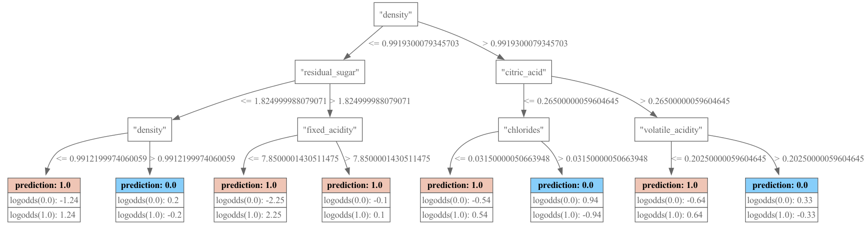
Tree models can be visualized by drawing their tree plots. For more examples, check out Machine Learning - Tree Plots.

model.plot_tree()

../_images/machine_learning_VAST_tree_gb_classifier_.png

Note

The above example may not render properly in the doc because of the huge size of the tree. But it should render nicely in jupyter environment.

In order to plot graph using graphviz separately, you can extract the graphviz DOT file code as follows:

model.to_graphviz()

This string can then be copied into a DOT file which can beparsed by graphviz.

Contour plot is another useful plot that can be produced for models with two predictors.

model.contour()

Important

Machine learning models with two predictors can usually benefit from their own contour plot. This visual representation aids in exploring predictions and gaining a deeper understanding of how these models perform in different scenarios. Please refer to Contour Plot for more examples.

Parameter Modification¶

In order to see the parameters:

model.get_params()

And to manually change some of the parameters:

model.set_params({'max_depth': 5})

Model Exporting¶

To Memmodel

model.to_memmodel()

Note

MemModel objects serve as in-memory representations of machine learning models. They can be used for both in-database and in-memory prediction tasks. These objects can be pickled in the same way that you would pickle a scikit-learn model.

The preceding methods for exporting the model use MemModel, and it is recommended to use MemModel directly.

To SQL

You can get the SQL query equivalent of the GradientBoosting model by:

model.to_sql()

Note

This SQL query can be directly used in any database.

Deploy SQL

To get the SQL query which uses VAST functions use below:

model.deploySQL()

To Python

To obtain the prediction function in Python syntax, use the following code:

X = [[4.2, 0.17, 0.36, 1.8, 0.029, 0.9899]]
model.to_python()(X)

Hint

The to_python() method is used to retrieve predictions, probabilities, or cluster distances. For specific details on how to use this method for different model types, refer to the relevant documentation for each model.

__init__(name: str = None, overwrite_model: bool = False, **kwargs) → None¶

Methods

`__init__`([name, overwrite_model])
`classification_report`([metrics, cutoff, ...])	Computes a classification report using multiple model evaluation metrics (`auc`, `accuracy`, `f1`...).
`confusion_matrix`([pos_label, cutoff])	Computes the model confusion matrix.
`contour`([pos_label, nbins, chart])	Draws the model's contour plot.
`cutoff_curve`([pos_label, nbins, show, chart])	Draws the model Cutoff curve.
`deploySQL`([X, pos_label, cutoff, allSQL])	Returns the SQL code needed to deploy the model.
`drop`()	Drops the model from the VAST DataBase.
`export_models`(name, path[, kind])	Exports machine learning models.
`features_importance`([tree_id, show, chart])	Computes the model's features importance.
`fit`(input_relation, X, y[, test_relation, ...])	Trains the model.
`get_attributes`([attr_name])	Returns the model attributes.
`get_match_index`(x, col_list[, str_check])	Returns the matching index.
`get_params`()	Returns the parameters of the model.
`get_plotting_lib`([class_name, chart, ...])	Returns the first available library (Plotly, Matplotlib) to draw a specific graphic.
`get_tree`([tree_id])	Returns a table with all the input tree information.
`import_models`(path[, schema, kind])	Imports machine learning models.
`lift_chart`([pos_label, nbins, show, chart])	Draws the model Lift Chart.
`plot`([max_nb_points, chart])	Draws the model.
`plot_tree`([tree_id, pic_path])	Draws the input tree.
`prc_curve`([pos_label, nbins, show, chart])	Draws the model PRC curve.
`predict`(vdf[, X, name, cutoff, inplace])	Predicts using the input relation.
`predict_proba`(vdf[, X, name, pos_label, inplace])	Returns the model's probabilities using the input relation.
`report`([metrics, cutoff, labels, nbins])	Computes a classification report using multiple model evaluation metrics (`auc`, `accuracy`, `f1`...).
`roc_curve`([pos_label, nbins, show, chart])	Draws the model ROC curve.
`score`([metric, average, pos_label, cutoff, ...])	Computes the model score.
`set_params`([parameters])	Sets the parameters of the model.
`summarize`()	Summarizes the model.
`to_binary`(path)	Exports the model to the VAST Binary format.
`to_graphviz`([tree_id, classes_color, ...])	Returns the code for a Graphviz tree.
`to_json`([path])	Creates a Python `GradientBoosting` JSON file that can be imported into the Python `GradientBoosting` API.
`to_memmodel`()	Converts the model to an InMemory object that can be used for different types of predictions.
`to_python`([return_proba, ...])	Returns the Python function needed for in-memory scoring without using built-in VAST functions.
`to_sql`([X, return_proba, ...])	Returns the SQL code needed to deploy the model without using built-in VAST functions.

Attributes

object_type