vastorbit.machine_learning.vast.cluster.BisectingKMeans

class vastorbit.machine_learning.vast.cluster.BisectingKMeans(name: str = None, overwrite_model: bool = False, **kwargs)

Creates a BisectingKMeans object using the VAST bisecting k-means algorithm. k-means clustering is a method of vector quantization, originally from signal processing, that aims to partition n observations into k clusters. Each observation belongs to the cluster with the nearest mean (cluster centers or cluster centroid), which serves as a prototype of the cluster. This results in a partitioning of the data space into Voronoi cells. Bisecting k-means combines k-means and hierarchical clustering.

Parameters:

• name (str, optional) – Name of the model. The model is stored in the database.

• overwrite_model (bool, optional) – If set to True, training a model with the same name as an existing model overwrites the existing model.

• **kwargs (scikit-learn model parameters.)

Variables:

• created (Many attributes are)

• phase. (during the fitting)

• feature_names_in_ (cluster_centers_, labels_, inertia_, n_features_in_,)

• note:: (..) – All attributes can be accessed using the get_attributes() method.

Examples

The following examples provide a basic understanding of usage. For more detailed examples, please refer to the Machine Learning or the Examples section on the website.

Load data for machine learning

We import vastorbit:

import vastorbit as vo

Hint

By assigning an alias to vastorbit, we mitigate the risk of code collisions with other libraries. This precaution is necessary because vastorbit uses commonly known function names like “average” and “median”, which can potentially lead to naming conflicts. The use of an alias ensures that the functions from vastorbit are used as intended without interfering with functions from other libraries.

For this example, we will use the winequality dataset.

import vastorbit.datasets as vod

data = vod.load_winequality()

	123 fixed_acidity Decimal(6, 3)	123 volatile_acidity Decimal(7, 4)	123 citric_acid Decimal(6, 3)	123 residual_sugar Decimal(7, 3)	123 chlorides Double	123 free_sulfur_dioxide Decimal(7, 2)	123 total_sulfur_dioxide Decimal(7, 2)	123 density Double	123 ph Decimal(6, 3)	123 sulphates Decimal(6, 3)	123 alcohol Double	123 quality Integer	123 good Integer	Abc color Varchar(20)
1	6.3	0.67	0.48	12.6	0.052	57.0	222.0	0.9979	3.17	0.52	9.3	6	0	white
2	7.4	0.4	0.29	5.4	0.044	31.0	122.0	0.994	3.3	0.5	11.1	8	1	white
3	7.1	0.26	0.31	2.2	0.044	29.0	128.0	0.9937	3.34	0.64	10.9	8	1	white
4	9.0	0.31	0.48	6.6	0.043	11.0	73.0	0.9938	2.9	0.38	11.6	5	0	white
5	6.3	0.39	0.24	6.9	0.069	9.0	117.0	0.9942	3.15	0.35	10.2	4	0	white
6	8.2	0.22	0.36	6.8	0.034	12.0	90.0	0.9944	3.01	0.38	10.5	8	1	white
7	7.1	0.19	0.28	3.6	0.033	16.0	78.0	0.993	2.91	0.78	11.4	6	0	white
8	7.3	0.25	0.36	13.1	0.05	35.0	200.0	0.9986	3.04	0.46	8.9	7	1	white
9	7.9	0.2	0.34	1.2	0.04	29.0	118.0	0.9932	3.14	0.41	10.6	6	0	white
10	7.1	0.26	0.32	5.9	0.037	39.0	97.0	0.9934	3.31	0.4	11.6	6	0	white
11	7.0	0.2	0.34	5.7	0.035	32.0	83.0	0.9928	3.19	0.46	11.5	6	0	white
12	6.9	0.3	0.33	4.1	0.035	26.0	155.0	0.9925	3.25	0.79	12.3	8	1	white
13	8.1	0.29	0.49	7.1	0.042	22.0	124.0	0.9944	3.14	0.41	10.8	6	0	white
14	5.8	0.17	0.3	1.4	0.037	55.0	130.0	0.9909	3.29	0.38	11.3	6	0	white
15	5.9	0.415	0.02	0.8	0.038	22.0	63.0	0.9932	3.36	0.36	9.3	5	0	white
16	6.6	0.23	0.26	1.3	0.045	16.0	128.0	0.9934	3.36	0.6	10.0	6	0	white
17	8.6	0.55	0.35	15.55	0.057	35.5	366.5	1.0001	3.04	0.63	11.0	3	0	white
18	6.9	0.35	0.74	1.0	0.044	18.0	132.0	0.992	3.13	0.55	10.2	5	0	white
19	7.6	0.14	0.74	1.6	0.04	27.0	103.0	0.9916	3.07	0.4	10.8	7	1	white
20	9.2	0.28	0.49	11.8	0.042	29.0	137.0	0.998	3.1	0.34	10.1	4	0	white
21	6.2	0.18	0.49	4.5	0.047	17.0	90.0	0.9919	3.27	0.37	11.6	6	0	white
22	5.3	0.165	0.24	1.1	0.051	25.0	105.0	0.9925	3.32	0.47	9.1	5	0	white
23	9.8	0.25	0.74	10.0	0.056	36.0	225.0	0.9977	3.06	0.43	10.0	4	0	white
24	8.1	0.29	0.49	7.1	0.042	22.0	124.0	0.9944	3.14	0.41	10.8	6	0	white
25	6.8	0.22	0.49	0.9	0.052	26.0	128.0	0.991	3.25	0.35	11.4	6	0	white
26	7.2	0.22	0.49	1.0	0.045	34.0	140.0	0.99	3.05	0.34	12.7	6	0	white
27	7.4	0.25	0.49	1.1	0.042	35.0	156.0	0.9917	3.13	0.55	11.3	5	0	white
28	8.2	0.18	0.49	1.1	0.033	28.0	81.0	0.9923	3.0	0.68	10.4	7	1	white
29	6.1	0.22	0.49	1.5	0.051	18.0	87.0	0.9928	3.3	0.46	9.6	5	0	white
30	7.0	0.39	0.24	1.0	0.048	8.0	119.0	0.9923	3.0	0.31	10.1	4	0	white
31	6.1	0.22	0.49	1.5	0.051	18.0	87.0	0.9928	3.3	0.46	9.6	5	0	white
32	6.5	0.36	0.49	2.9	0.03	16.0	94.0	0.9902	3.1	0.49	12.1	7	1	white
33	7.1	0.29	0.49	1.2	0.031	32.0	99.0	0.9893	3.07	0.33	12.2	6	0	white
34	7.4	0.25	0.49	1.1	0.042	35.0	156.0	0.9917	3.13	0.55	11.3	5	0	white
35	6.9	0.23	0.24	14.2	0.053	19.0	94.0	0.9982	3.17	0.5	9.6	5	0	white
36	8.5	0.56	0.74	17.85	0.051	51.0	243.0	1.0005	2.99	0.7	9.2	5	0	white
37	8.2	0.18	0.49	1.1	0.033	28.0	81.0	0.9923	3.0	0.68	10.4	7	1	white
38	6.3	0.23	0.49	7.1	0.05	67.0	210.0	0.9951	3.23	0.34	9.5	5	0	white
39	6.1	0.25	0.49	7.6	0.052	67.0	226.0	0.9956	3.16	0.47	8.9	5	0	white
40	7.2	0.26	0.74	13.6	0.05	56.0	162.0	0.998	3.03	0.44	8.8	5	0	white
41	7.2	0.31	0.24	1.4	0.057	17.0	117.0	0.9928	3.16	0.35	10.5	5	0	white
42	8.0	0.25	0.49	1.2	0.061	27.0	117.0	0.9938	3.08	0.34	9.4	5	0	white
43	7.0	0.18	0.49	5.3	0.04	34.0	125.0	0.9914	3.24	0.4	12.2	6	0	white
44	7.8	0.43	0.49	13.0	0.033	37.0	158.0	0.9955	3.14	0.35	11.3	6	0	white
45	8.3	0.2	0.74	4.45	0.044	33.0	130.0	0.9924	3.25	0.42	12.2	6	0	white
46	6.3	0.27	0.49	1.2	0.063	35.0	92.0	0.9911	3.38	0.42	12.2	6	0	white
47	7.4	0.16	0.49	1.2	0.055	18.0	150.0	0.9917	3.23	0.47	11.2	6	0	white
48	7.4	0.16	0.49	1.2	0.055	18.0	150.0	0.9917	3.23	0.47	11.2	6	0	white
49	6.9	0.19	0.49	6.6	0.036	49.0	172.0	0.9932	3.2	0.27	11.5	6	0	white
50	7.8	0.43	0.49	13.0	0.033	37.0	158.0	0.9955	3.14	0.35	11.3	6	0	white
51	7.2	0.4	0.49	1.1	0.048	11.0	138.0	0.9929	3.01	0.42	9.3	5	0	white
52	7.8	0.43	0.49	13.0	0.033	37.0	158.0	0.9955	3.14	0.35	11.3	6	0	white
53	7.6	0.52	0.49	14.0	0.034	37.0	156.0	0.9958	3.14	0.38	11.8	7	1	white
54	8.3	0.21	0.49	19.8	0.054	50.0	231.0	1.0012	2.99	0.54	9.2	5	0	white
55	6.9	0.34	0.74	11.2	0.069	44.0	150.0	0.9968	3.0	0.81	9.2	5	0	white
56	6.3	0.27	0.49	1.2	0.063	35.0	92.0	0.9911	3.38	0.42	12.2	6	0	white
57	8.3	0.2	0.74	4.45	0.044	33.0	130.0	0.9924	3.25	0.42	12.2	6	0	white
58	7.1	0.22	0.74	2.7	0.044	42.0	144.0	0.991	3.31	0.41	12.2	6	0	white
59	7.9	0.11	0.49	4.5	0.048	27.0	133.0	0.9946	3.24	0.42	10.6	6	0	white
60	8.5	0.17	0.74	3.6	0.05	29.0	128.0	0.9928	3.28	0.4	12.4	6	0	white
61	6.4	0.145	0.49	5.4	0.048	54.0	164.0	0.9946	3.56	0.44	10.8	6	0	white
62	7.4	0.16	0.49	1.2	0.055	18.0	150.0	0.9917	3.23	0.47	11.2	6	0	white
63	8.3	0.19	0.49	1.2	0.051	11.0	137.0	0.9918	3.06	0.46	11.0	6	0	white
64	8.0	0.44	0.49	9.1	0.031	46.0	151.0	0.9926	3.16	0.27	12.7	8	1	white
65	7.0	0.2	0.74	0.8	0.044	19.0	163.0	0.9931	3.46	0.53	10.2	5	0	white
66	6.9	0.19	0.49	6.6	0.036	49.0	172.0	0.9932	3.2	0.27	11.5	6	0	white
67	7.1	0.25	0.49	3.0	0.03	30.0	96.0	0.9903	3.13	0.39	12.3	7	1	white
68	6.5	0.24	0.24	1.6	0.046	15.0	60.0	0.9928	3.19	0.39	9.8	5	0	white
69	7.2	0.4	0.49	1.1	0.048	11.0	138.0	0.9929	3.01	0.42	9.3	5	0	white
70	7.6	0.52	0.49	14.0	0.034	37.0	156.0	0.9958	3.14	0.38	11.8	7	1	white
71	7.8	0.43	0.49	13.0	0.033	37.0	158.0	0.9955	3.14	0.35	11.3	6	0	white
72	7.8	0.21	0.49	1.35	0.052	6.0	48.0	0.9911	3.15	0.28	11.4	5	0	white
73	7.0	0.2	0.49	5.9	0.038	39.0	128.0	0.9938	3.21	0.48	10.8	6	0	white
74	6.9	0.25	0.24	3.6	0.057	13.0	85.0	0.9942	2.99	0.48	9.5	4	0	white
75	7.2	0.08	0.49	1.3	0.05	18.0	148.0	0.9945	3.46	0.44	10.2	6	0	white
76	7.1	0.85	0.49	8.7	0.028	40.0	184.0	0.9962	3.22	0.36	10.7	5	0	white
77	7.6	0.51	0.24	1.2	0.04	10.0	104.0	0.992	3.05	0.29	10.8	6	0	white
78	7.9	0.22	0.24	4.6	0.044	39.0	159.0	0.9927	2.99	0.28	11.5	6	0	white
79	7.7	0.16	0.49	2.0	0.056	20.0	124.0	0.9948	3.32	0.49	10.7	6	0	white
80	7.2	0.08	0.49	1.3	0.05	18.0	148.0	0.9945	3.46	0.44	10.2	6	0	white
81	6.6	0.25	0.24	1.7	0.048	26.0	124.0	0.9942	3.37	0.6	10.1	6	0	white
82	6.7	0.16	0.49	2.4	0.046	57.0	187.0	0.9952	3.62	0.81	10.4	6	0	white
83	6.9	0.25	0.24	3.6	0.057	13.0	85.0	0.9942	2.99	0.48	9.5	4	0	white
84	7.5	0.32	0.24	4.6	0.053	8.0	134.0	0.9958	3.14	0.5	9.1	3	0	white
85	7.4	0.28	0.49	1.5	0.034	20.0	126.0	0.9918	2.98	0.39	10.6	6	0	white
86	6.2	0.15	0.49	0.9	0.033	17.0	51.0	0.9932	3.3	0.7	9.4	6	0	white
87	6.7	0.25	0.74	19.4	0.054	44.0	169.0	1.0004	3.51	0.45	9.8	6	0	white
88	6.5	0.26	0.74	13.3	0.044	68.0	224.0	0.9972	3.18	0.54	9.5	6	0	white
89	7.9	0.16	0.74	17.85	0.037	52.0	187.0	0.9998	2.99	0.41	9.3	5	0	white
90	5.6	0.185	0.49	1.1	0.03	28.0	117.0	0.9918	3.55	0.45	10.3	6	0	white
91	7.5	0.2	0.49	1.3	0.031	8.0	97.0	0.9918	3.06	0.62	11.1	5	0	white
92	8.0	0.3	0.49	9.4	0.046	47.0	188.0	0.9964	3.14	0.48	10.0	5	0	white
93	8.0	0.34	0.49	9.0	0.033	39.0	180.0	0.9936	3.13	0.38	12.3	8	1	white
94	7.7	0.35	0.49	8.65	0.033	42.0	186.0	0.9931	3.14	0.38	12.4	8	1	white
95	7.6	0.29	0.49	9.6	0.03	45.0	197.0	0.9938	3.13	0.38	12.3	7	1	white
96	6.7	0.62	0.24	1.1	0.039	6.0	62.0	0.9934	3.41	0.32	10.4	5	0	white
97	6.8	0.27	0.49	1.2	0.044	35.0	126.0	0.99	3.13	0.48	12.1	7	1	white
98	7.7	0.27	0.49	1.8	0.041	23.0	86.0	0.9914	3.16	0.42	12.5	6	0	white
99	6.7	0.51	0.24	2.1	0.043	14.0	155.0	0.9904	3.22	0.6	13.0	6	0	white
100	7.4	0.19	0.49	9.3	0.03	26.0	132.0	0.994	2.99	0.32	11.0	7	1	white

Rows: 1-100 | Columns: 14

Note

vastorbit offers a wide range of sample datasets that are ideal for training and testing purposes. You can explore the full list of available datasets in the Datasets, which provides detailed information on each dataset and how to use them effectively. These datasets are invaluable resources for honing your data analysis and machine learning skills within the vastorbit environment.

Model Initialization

First we import the BisectingKMeans model:

from vastorbit.machine_learning.vast import BisectingKMeans

Then we can create the model:

model = BisectingKMeans(
    n_clusters = 8,
    algorithm = 'lloyd',
    bisecting_strategy = "biggest_inertia",
    max_iter = 300,
    tol = 1e-4,
)

Important

The model name is crucial for the model management system and versioning. It’s highly recommended to provide a name if you plan to reuse the model later.

Model Training

We can now fit the model:

model.fit(data, X = ["density", "sulphates"])

Important

To train a model, you can directly use the VastFrame or the name of the relation stored in the database. The test set is optional and is only used to compute the test metrics. In vastorbit, we don’t work using X matrices and y vectors. Instead, we work directly with lists of predictors and the response name.

Hint

For clustering and anomaly detection, the use of predictors is optional. In such cases, all available predictors are considered, which can include solely numerical variables or a combination of numerical and categorical variables, depending on the model’s capabilities.

Metrics

You can also find the cluster positions by:

model.clusters_

In order to get the size of each cluster, you can use:

model.cluster_size_

To evaluate the model, various attributes are computed, such as the between sum of squares, the total within clusters sum of squares, and the total sum of squares.

model.between_clusters_ss_
model.total_within_clusters_ss_
model.total_ss_

You also have access to the sum of squares of each cluster.

model.cluster_i_ss_

Some other useful attributes can be used to evaluate the model, like the Elbow Score (the bigger it is, the better it is).

model.elbow_score_

Prediction

Predicting or ranking the dataset is straight-forward:

model.predict(data, ["density", "sulphates"])

	123 fixed_acidity Decimal(6, 3)	123 volatile_acidity Decimal(7, 4)	123 citric_acid Decimal(6, 3)	123 residual_sugar Decimal(7, 3)	123 chlorides Double	123 free_sulfur_dioxide Decimal(7, 2)	123 total_sulfur_dioxide Decimal(7, 2)	123 density Double	123 ph Decimal(6, 3)	123 sulphates Decimal(6, 3)	123 alcohol Double	123 quality Integer	123 good Integer	Abc color Varchar(20)	123 BisectingKMeans_defaultvastorbittmpbisectingkmeansmemoryadmin9921f18e754811f1becdea8c65480234 Integer
1	6.3	0.67	0.48	12.6	0.052	57.0	222.0	0.9979	3.17	0.52	9.3	6	0	white	6
2	7.4	0.4	0.29	5.4	0.044	31.0	122.0	0.994	3.3	0.5	11.1	8	1	white	6
3	7.1	0.26	0.31	2.2	0.044	29.0	128.0	0.9937	3.34	0.64	10.9	8	1	white	6
4	9.0	0.31	0.48	6.6	0.043	11.0	73.0	0.9938	2.9	0.38	11.6	5	0	white	6
5	6.3	0.39	0.24	6.9	0.069	9.0	117.0	0.9942	3.15	0.35	10.2	4	0	white	6
6	8.2	0.22	0.36	6.8	0.034	12.0	90.0	0.9944	3.01	0.38	10.5	8	1	white	6
7	7.1	0.19	0.28	3.6	0.033	16.0	78.0	0.993	2.91	0.78	11.4	6	0	white	6
8	7.3	0.25	0.36	13.1	0.05	35.0	200.0	0.9986	3.04	0.46	8.9	7	1	white	6
9	7.9	0.2	0.34	1.2	0.04	29.0	118.0	0.9932	3.14	0.41	10.6	6	0	white	6
10	7.1	0.26	0.32	5.9	0.037	39.0	97.0	0.9934	3.31	0.4	11.6	6	0	white	6
11	7.0	0.2	0.34	5.7	0.035	32.0	83.0	0.9928	3.19	0.46	11.5	6	0	white	6
12	6.9	0.3	0.33	4.1	0.035	26.0	155.0	0.9925	3.25	0.79	12.3	8	1	white	6
13	8.1	0.29	0.49	7.1	0.042	22.0	124.0	0.9944	3.14	0.41	10.8	6	0	white	6
14	5.8	0.17	0.3	1.4	0.037	55.0	130.0	0.9909	3.29	0.38	11.3	6	0	white	6
15	5.9	0.415	0.02	0.8	0.038	22.0	63.0	0.9932	3.36	0.36	9.3	5	0	white	6
16	6.6	0.23	0.26	1.3	0.045	16.0	128.0	0.9934	3.36	0.6	10.0	6	0	white	6
17	8.6	0.55	0.35	15.55	0.057	35.5	366.5	1.0001	3.04	0.63	11.0	3	0	white	6
18	6.9	0.35	0.74	1.0	0.044	18.0	132.0	0.992	3.13	0.55	10.2	5	0	white	6
19	7.6	0.14	0.74	1.6	0.04	27.0	103.0	0.9916	3.07	0.4	10.8	7	1	white	6
20	9.2	0.28	0.49	11.8	0.042	29.0	137.0	0.998	3.1	0.34	10.1	4	0	white	6
21	6.2	0.18	0.49	4.5	0.047	17.0	90.0	0.9919	3.27	0.37	11.6	6	0	white	6
22	5.3	0.165	0.24	1.1	0.051	25.0	105.0	0.9925	3.32	0.47	9.1	5	0	white	6
23	9.8	0.25	0.74	10.0	0.056	36.0	225.0	0.9977	3.06	0.43	10.0	4	0	white	6
24	8.1	0.29	0.49	7.1	0.042	22.0	124.0	0.9944	3.14	0.41	10.8	6	0	white	6
25	6.8	0.22	0.49	0.9	0.052	26.0	128.0	0.991	3.25	0.35	11.4	6	0	white	6
26	7.2	0.22	0.49	1.0	0.045	34.0	140.0	0.99	3.05	0.34	12.7	6	0	white	6
27	7.4	0.25	0.49	1.1	0.042	35.0	156.0	0.9917	3.13	0.55	11.3	5	0	white	6
28	8.2	0.18	0.49	1.1	0.033	28.0	81.0	0.9923	3.0	0.68	10.4	7	1	white	6
29	6.1	0.22	0.49	1.5	0.051	18.0	87.0	0.9928	3.3	0.46	9.6	5	0	white	6
30	7.0	0.39	0.24	1.0	0.048	8.0	119.0	0.9923	3.0	0.31	10.1	4	0	white	6
31	6.1	0.22	0.49	1.5	0.051	18.0	87.0	0.9928	3.3	0.46	9.6	5	0	white	6
32	6.5	0.36	0.49	2.9	0.03	16.0	94.0	0.9902	3.1	0.49	12.1	7	1	white	6
33	7.1	0.29	0.49	1.2	0.031	32.0	99.0	0.9893	3.07	0.33	12.2	6	0	white	6
34	7.4	0.25	0.49	1.1	0.042	35.0	156.0	0.9917	3.13	0.55	11.3	5	0	white	6
35	6.9	0.23	0.24	14.2	0.053	19.0	94.0	0.9982	3.17	0.5	9.6	5	0	white	6
36	8.5	0.56	0.74	17.85	0.051	51.0	243.0	1.0005	2.99	0.7	9.2	5	0	white	6
37	8.2	0.18	0.49	1.1	0.033	28.0	81.0	0.9923	3.0	0.68	10.4	7	1	white	6
38	6.3	0.23	0.49	7.1	0.05	67.0	210.0	0.9951	3.23	0.34	9.5	5	0	white	6
39	6.1	0.25	0.49	7.6	0.052	67.0	226.0	0.9956	3.16	0.47	8.9	5	0	white	6
40	7.2	0.26	0.74	13.6	0.05	56.0	162.0	0.998	3.03	0.44	8.8	5	0	white	6
41	7.2	0.31	0.24	1.4	0.057	17.0	117.0	0.9928	3.16	0.35	10.5	5	0	white	6
42	8.0	0.25	0.49	1.2	0.061	27.0	117.0	0.9938	3.08	0.34	9.4	5	0	white	6
43	7.0	0.18	0.49	5.3	0.04	34.0	125.0	0.9914	3.24	0.4	12.2	6	0	white	6
44	7.8	0.43	0.49	13.0	0.033	37.0	158.0	0.9955	3.14	0.35	11.3	6	0	white	6
45	8.3	0.2	0.74	4.45	0.044	33.0	130.0	0.9924	3.25	0.42	12.2	6	0	white	6
46	6.3	0.27	0.49	1.2	0.063	35.0	92.0	0.9911	3.38	0.42	12.2	6	0	white	6
47	7.4	0.16	0.49	1.2	0.055	18.0	150.0	0.9917	3.23	0.47	11.2	6	0	white	6
48	7.4	0.16	0.49	1.2	0.055	18.0	150.0	0.9917	3.23	0.47	11.2	6	0	white	6
49	6.9	0.19	0.49	6.6	0.036	49.0	172.0	0.9932	3.2	0.27	11.5	6	0	white	6
50	7.8	0.43	0.49	13.0	0.033	37.0	158.0	0.9955	3.14	0.35	11.3	6	0	white	6
51	7.2	0.4	0.49	1.1	0.048	11.0	138.0	0.9929	3.01	0.42	9.3	5	0	white	6
52	7.8	0.43	0.49	13.0	0.033	37.0	158.0	0.9955	3.14	0.35	11.3	6	0	white	6
53	7.6	0.52	0.49	14.0	0.034	37.0	156.0	0.9958	3.14	0.38	11.8	7	1	white	6
54	8.3	0.21	0.49	19.8	0.054	50.0	231.0	1.0012	2.99	0.54	9.2	5	0	white	6
55	6.9	0.34	0.74	11.2	0.069	44.0	150.0	0.9968	3.0	0.81	9.2	5	0	white	6
56	6.3	0.27	0.49	1.2	0.063	35.0	92.0	0.9911	3.38	0.42	12.2	6	0	white	6
57	8.3	0.2	0.74	4.45	0.044	33.0	130.0	0.9924	3.25	0.42	12.2	6	0	white	6
58	7.1	0.22	0.74	2.7	0.044	42.0	144.0	0.991	3.31	0.41	12.2	6	0	white	6
59	7.9	0.11	0.49	4.5	0.048	27.0	133.0	0.9946	3.24	0.42	10.6	6	0	white	6
60	8.5	0.17	0.74	3.6	0.05	29.0	128.0	0.9928	3.28	0.4	12.4	6	0	white	6
61	6.4	0.145	0.49	5.4	0.048	54.0	164.0	0.9946	3.56	0.44	10.8	6	0	white	6
62	7.4	0.16	0.49	1.2	0.055	18.0	150.0	0.9917	3.23	0.47	11.2	6	0	white	6
63	8.3	0.19	0.49	1.2	0.051	11.0	137.0	0.9918	3.06	0.46	11.0	6	0	white	6
64	8.0	0.44	0.49	9.1	0.031	46.0	151.0	0.9926	3.16	0.27	12.7	8	1	white	6
65	7.0	0.2	0.74	0.8	0.044	19.0	163.0	0.9931	3.46	0.53	10.2	5	0	white	6
66	6.9	0.19	0.49	6.6	0.036	49.0	172.0	0.9932	3.2	0.27	11.5	6	0	white	6
67	7.1	0.25	0.49	3.0	0.03	30.0	96.0	0.9903	3.13	0.39	12.3	7	1	white	6
68	6.5	0.24	0.24	1.6	0.046	15.0	60.0	0.9928	3.19	0.39	9.8	5	0	white	6
69	7.2	0.4	0.49	1.1	0.048	11.0	138.0	0.9929	3.01	0.42	9.3	5	0	white	6
70	7.6	0.52	0.49	14.0	0.034	37.0	156.0	0.9958	3.14	0.38	11.8	7	1	white	6
71	7.8	0.43	0.49	13.0	0.033	37.0	158.0	0.9955	3.14	0.35	11.3	6	0	white	6
72	7.8	0.21	0.49	1.35	0.052	6.0	48.0	0.9911	3.15	0.28	11.4	5	0	white	6
73	7.0	0.2	0.49	5.9	0.038	39.0	128.0	0.9938	3.21	0.48	10.8	6	0	white	6
74	6.9	0.25	0.24	3.6	0.057	13.0	85.0	0.9942	2.99	0.48	9.5	4	0	white	6
75	7.2	0.08	0.49	1.3	0.05	18.0	148.0	0.9945	3.46	0.44	10.2	6	0	white	6
76	7.1	0.85	0.49	8.7	0.028	40.0	184.0	0.9962	3.22	0.36	10.7	5	0	white	6
77	7.6	0.51	0.24	1.2	0.04	10.0	104.0	0.992	3.05	0.29	10.8	6	0	white	6
78	7.9	0.22	0.24	4.6	0.044	39.0	159.0	0.9927	2.99	0.28	11.5	6	0	white	6
79	7.7	0.16	0.49	2.0	0.056	20.0	124.0	0.9948	3.32	0.49	10.7	6	0	white	6
80	7.2	0.08	0.49	1.3	0.05	18.0	148.0	0.9945	3.46	0.44	10.2	6	0	white	6
81	6.6	0.25	0.24	1.7	0.048	26.0	124.0	0.9942	3.37	0.6	10.1	6	0	white	6
82	6.7	0.16	0.49	2.4	0.046	57.0	187.0	0.9952	3.62	0.81	10.4	6	0	white	6
83	6.9	0.25	0.24	3.6	0.057	13.0	85.0	0.9942	2.99	0.48	9.5	4	0	white	6
84	7.5	0.32	0.24	4.6	0.053	8.0	134.0	0.9958	3.14	0.5	9.1	3	0	white	6
85	7.4	0.28	0.49	1.5	0.034	20.0	126.0	0.9918	2.98	0.39	10.6	6	0	white	6
86	6.2	0.15	0.49	0.9	0.033	17.0	51.0	0.9932	3.3	0.7	9.4	6	0	white	6
87	6.7	0.25	0.74	19.4	0.054	44.0	169.0	1.0004	3.51	0.45	9.8	6	0	white	6
88	6.5	0.26	0.74	13.3	0.044	68.0	224.0	0.9972	3.18	0.54	9.5	6	0	white	6
89	7.9	0.16	0.74	17.85	0.037	52.0	187.0	0.9998	2.99	0.41	9.3	5	0	white	6
90	5.6	0.185	0.49	1.1	0.03	28.0	117.0	0.9918	3.55	0.45	10.3	6	0	white	6
91	7.5	0.2	0.49	1.3	0.031	8.0	97.0	0.9918	3.06	0.62	11.1	5	0	white	6
92	8.0	0.3	0.49	9.4	0.046	47.0	188.0	0.9964	3.14	0.48	10.0	5	0	white	6
93	8.0	0.34	0.49	9.0	0.033	39.0	180.0	0.9936	3.13	0.38	12.3	8	1	white	6
94	7.7	0.35	0.49	8.65	0.033	42.0	186.0	0.9931	3.14	0.38	12.4	8	1	white	6
95	7.6	0.29	0.49	9.6	0.03	45.0	197.0	0.9938	3.13	0.38	12.3	7	1	white	6
96	6.7	0.62	0.24	1.1	0.039	6.0	62.0	0.9934	3.41	0.32	10.4	5	0	white	6
97	6.8	0.27	0.49	1.2	0.044	35.0	126.0	0.99	3.13	0.48	12.1	7	1	white	6
98	7.7	0.27	0.49	1.8	0.041	23.0	86.0	0.9914	3.16	0.42	12.5	6	0	white	6
99	6.7	0.51	0.24	2.1	0.043	14.0	155.0	0.9904	3.22	0.6	13.0	6	0	white	6
100	7.4	0.19	0.49	9.3	0.03	26.0	132.0	0.994	2.99	0.32	11.0	7	1	white	6

Rows: 1-100 | Columns: 15

As shown above, a new column has been created, containing the bisected clusters.

Plots - Cluster Plot

Plots highlighting the different clusters can be easily drawn using:

model.plot()

Plots - Tree

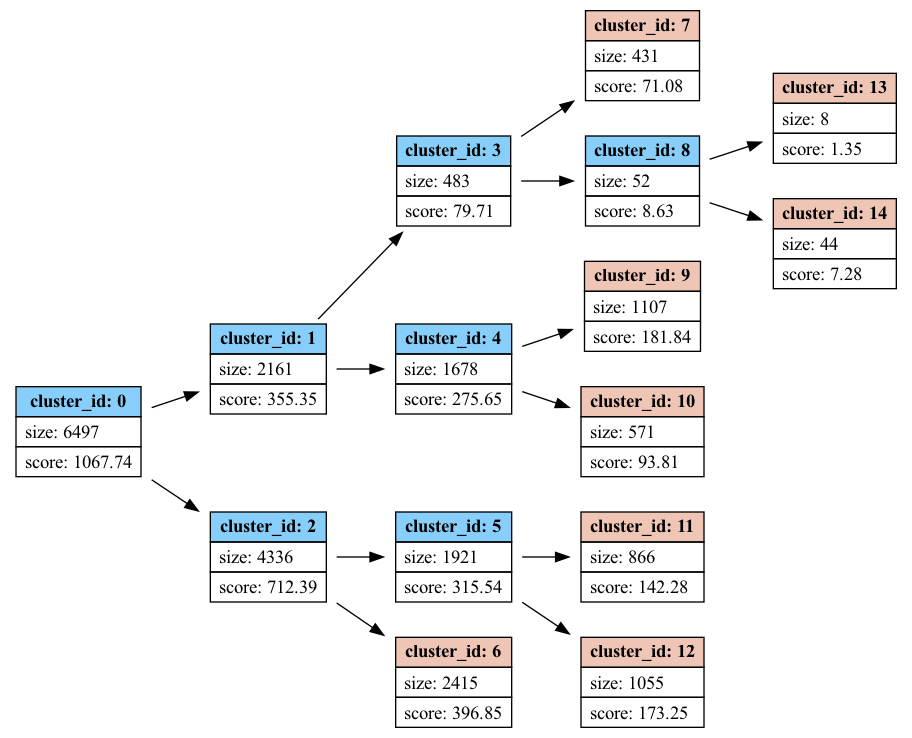
Tree models can be visualized by drawing their tree plots. For more examples, check out Machine Learning - Tree Plots.

model.plot_tree()

Note

The above example may not render properly in the doc because of the huge size of the tree. But it should render nicely in jupyter environment.

In order to plot graph using graphviz separately, you can extract the graphviz DOT file code as follows:

model.to_graphviz()

This string can then be copied into a DOT file which can be parsed by graphviz.

Plots - Contour

In order to understand the parameter space, we can also look at the contour plots:

model.contour()

Note

Machine learning models with two predictors can usually benefit from their own contour plot. This visual representation aids in exploring predictions and gaining a deeper understanding of how these models perform in different scenarios. Please refer to Contour Plot for more examples.

Parameter Modification

In order to see the parameters:

model.get_params()

And to manually change some of the parameters:

model.set_params({'n_clusters': 5})

Model Exporting

To Memmodel

model.to_memmodel()

Note

MemModel objects serve as in-memory representations of machine learning models. They can be used for both in-database and in-memory prediction tasks. These objects can be pickled in the same way that you would pickle a scikit-learn model.

The preceding methods for exporting the model use MemModel, and it is recommended to use MemModel directly.

To SQL

You can get the SQL query equivalent of the GB model by:

model.to_sql()

Note

This SQL query can be directly used in any database.

Deploy SQL

To get the SQL query which uses VAST functions use below:

model.deploySQL()

To Python

To obtain the prediction function in Python syntax, use the following code:

X = [[0.9, 0.5]]
model.to_python()(X)

Hint

The to_python() method is used to retrieve the anomaly score. For specific details on how to use this method for different model types, refer to the relevant documentation for each model.

__init__(name: str = None, overwrite_model: bool = False, **kwargs) → None

Methods

__init__([name, overwrite_model])
contour([nbins, chart])	Draws the model's contour plot.
deploySQL([X])	Returns the SQL code needed to deploy the model.
drop()	Drops the model from the VAST DataBase.
export_models(name, path[, kind])	Exports machine learning models.
features_importance([tree_id, show, chart])	Computes the model's features importance.
fit(input_relation[, X, return_report])	Trains the model.
get_attributes([attr_name])	Returns the model attributes.
get_match_index(x, col_list[, str_check])	Returns the matching index.
get_params()	Returns the parameters of the model.
get_plotting_lib([class_name, chart, ...])	Returns the first available library (Plotly, Matplotlib) to draw a specific graphic.
get_tree()	Returns a table containing information about the BK-tree.
import_models(path[, schema, kind])	Imports machine learning models.
plot([max_nb_points, chart])	Draws the model.
plot_tree([pic_path])	Draws the input tree.
plot_voronoi([max_nb_points, plot_crosses, ...])	Draws the Voronoi Graph of the model.
predict(vdf[, X, name, inplace])	Makes predictions using the input relation.
set_params([parameters])	Sets the parameters of the model.
summarize()	Summarizes the model.
to_binary(path)	Exports the model to the VAST Binary format.
to_graphviz([round_score, percent, ...])	Returns the code for a Graphviz tree.
to_memmodel()	Converts the model to an InMemory object that can be used for different types of predictions.
to_python([return_proba, ...])	Returns the Python function needed for in-memory scoring without using built-in VAST functions.
to_sql([X, return_proba, ...])	Returns the SQL code needed to deploy the model without using built-in VAST functions.

Attributes

object_type